Time-Harmonic Maxwell#
This subsection describes the parameters for the time-harmonic Maxwell solver, a
Discontinuous Petrov-Galerkin (DPG) formulation for time-harmonic electromagnetic
problems, i.e., problems in which the fields oscillate at a single, fixed frequency
and are represented by their complex-valued phasor amplitudes. These parameters are
declared in the time harmonic maxwell subsection of the parameter file.
Attention
The time-harmonic Maxwell solver currently supports 3D problems only.
Before detailing the parameters, we first describe the non-dimensionalization convention used internally by the solver, since some parameters (e.g., the field amplitudes) are defined with respect to it.
Dimensionless Formulation#
The solver always works internally in dimensionless form, and rescales the solution
back to physical units only at the end, according to the selected
electromagnetic scaling type. The system of equations is non-dimensionalized
using the following conventions:
where
\(E_0\) is the reference electric-field amplitude, set via
electric field amplitude,\(Z_0 = \sqrt{\mu_0/\varepsilon_0}\) is the impedance of free space,
\(L\) is the reference length scale of the mesh,
\(c_0\) is the speed of light in vacuum,
\(\varepsilon_0\) and \(\mu_0\) are the permittivity and permeability of vacuum,
\(\varepsilon\), \(\mu\), and \(\sigma\) are the (dimensional) permittivity, permeability, and electrical conductivity of the medium, and
\(\omega\) is the (dimensional) angular frequency, set internally from the
electromagnetic frequencyparameter.
Using these conventions, the time-harmonic Maxwell system is written in dimensionless form (using the time-harmonic ansatz \(\mathbf{E}(\mathbf{x},t) = \Re(\mathbf{E}_\mathrm{spatial}(\mathbf{x})e^{-i\omega t})\)) as:
where \(\tilde{\mathbf{E}}\) and \(\tilde{\mathbf{H}}\) are the dimensionless electric and magnetic fields, \(\tilde{\omega}\) is the dimensionless angular frequency, \(\mu_r\) is the relative magnetic permeability, and \(\tilde{\mathbf{J}}\) is the dimensionless current density.
Note
The effective relative permittivity \(\varepsilon_{r,\text{eff}}\) combines the medium’s relative permittivity \(\varepsilon_r\) with its conductive losses \(\sigma_r\) into a single complex coefficient via the relation \(\varepsilon_{r,\text{eff}} = \varepsilon_r + i \sigma_r\).
Tip
If the user wants to use different units than the MKS system because, for example, the problem is defined in centimeters, we recommend using the dimensionality subsection to set the reference length scale \(L\) to 0.01 m, and leave all the parameters in the PRM file in MKS units. The solver will then automatically convert the parameters to the correct dimensionless form. If not using the dimensionality subsection, the user must ensure that all parameters are consistent with the desired behavior following the conventions described above.
Parameter File Syntax#
An example of the time-harmonic Maxwell parameters is given in the text box below.
subsection time harmonic maxwell

  set electromagnetic frequency    = 1 # Hz

  set electromagnetic scaling type = <none|electric_field|magnetic_field|power>

  set electric field amplitude     = 1
  set magnetic field amplitude     = 1

  set number of waveguide inlets   = 0

  # The block below illustrates the syntax of a waveguide inlet subsection.
  # It is only parsed if "number of waveguide inlets" is at least 1.
  subsection waveguide inlet 0
    set port boundary id = 0
    set waveguide power  = 1 # Watts

    subsection waveguide mode
      set mode type    = <TE|TM>
      set mode order m = 1
      set mode order n = 0
    end

    set corner 0 = 0,0,0
    set corner 1 = 1,0,0
    set corner 2 = 0,1,0
    set corner 3 = 1,1,0
  end

  subsection time coupling strategy
    set type               = <none|iteration|time|threshold>
    set coupling iteration = 1
    set coupling time      = 1
    set coupling threshold = 0.1
  end
end
Note
The number of waveguide inlets is at most 10, and the inlets are numbered
from 0 to 9. Their properties are defined in the waveguide inlet i
subsections, where i is the inlet number. At the moment, all inlets need to
have the same frequency, which is set in the parent
time harmonic maxwell subsection, as the solver does not support solving
for multiple frequencies at the same time.
electromagnetic frequency: excitation frequency of the time-harmonic wave, in Hz. This is required for any time-harmonic Maxwell problem.electromagnetic scaling type: selects how the solution is rescaled back to physical units after the linear system is solved. The choices are:none(default): the solution is left in dimensionless form and output as such.electric_field: rescaled so the electric field matcheselectric field amplitude, and the magnetic field matches \(H_0 = E_0 / Z_0\).magnetic_field: rescaled so the magnetic field matchesmagnetic field amplitude, and the electric field matches \(E_0 = Z_0 H_0\).power: rescaled so the power delivered through the waveguide inlet matches thewaveguide powergiven in watts by the user for that inlet. The scaling is done internally by isolating the electric field amplitude using the Poynting vector and the waveguide mode properties, and then rescaling the magnetic field accordingly, via the relation:\[\overline{P}_\text{input} = \frac{1}{2} \frac{E_0^2}{Z_0} \int_A \Re{(\mathbf{E} \times \mathbf{H}^*)} \cdot \mathbf{n} \text{d}A,\]where \(\overline{P}_\text{input}\) is the input power defined by the user, \(E_0\) is the electric field amplitude, \(Z_0\) is the impedance of free space, and the integral is taken over the waveguide inlet area \(A\). The Poynting vector is computed using the electric and magnetic fields of the selected waveguide mode.
Attention
Setting
electromagnetic scaling type = powerrequiresnumber of waveguide inletsto be at least 1, since there would otherwise be no waveguide power to normalize against.Warning
The
electromagnetic scaling typeparameter only rescales the solution back to physical units after the linear system is solved; it does not affect the non-dimensionalization of the equations, which always uses the reference electric-field amplitude \(E_0\) and the impedance of free space \(Z_0\). However, in multiphysics simulations, the scaling type must not benoneif the electromagnetic fields are to be coupled to other physics, since the other physics expect dimensional fields.electric field amplitude: the reference amplitude \(E_0\) used as the target amplitude whenelectromagnetic scaling type = electric_field.magnetic field amplitude: the reference amplitude \(H_0 = E_0 / Z_0\) used as the target amplitude whenelectromagnetic scaling type = magnetic_field.number of waveguide inlets: number ofwaveguide inletsubsections to apply on the geometry boundary. See also the boundary conditions section for more information on the waveguide boundary conditions.
Waveguide Inlets#
Each waveguide inlet i subsection describes one rectangular waveguide port
through which a mode is excited, where i is the inlet number (0 to
9).
Note
At the moment only rectangular waveguide modes are supported, and the user must ensure that the selected mode is valid according to the waveguide geometry.
port boundary id: the boundary id of the mesh on which the inlet is applied.waveguide power: excitation power in Watts of the waveguide inlet. This is used to rescale the solution back to physical units whenelectromagnetic scaling type = power.
Waveguide Mode#
The subsection waveguide mode defines the rectangular waveguide mode
excited at the inlet.
mode type:TE(default) orTM, standing for transverse electric or transverse magnetic, respectively. TheTEmode is defined by the following equations:\[\begin{split}\begin{align} \mathbf{E}_{TE} & = i\frac{\omega \mu_r}{k_c^2} \begin{bmatrix} -k_{x_2} \cos(k_{x_1} x_1) \sin(k_{x_2} x_2) \\ k_{x_1} \sin(k_{x_1} x_1) \cos(k_{x_2} x_2) \\ 0 \end{bmatrix} e^{i k_{x_3} x_3}, \\ \mathbf{H}_{TE} & = \begin{bmatrix} - i \frac{k_{x_3} k_{x_1}}{k_c^2} \sin(k_{x_1} x_1) \cos(k_{x_2} x_2) \\-i \frac{k_{x_3} k_{x_2}}{k_c^2} \cos(k_{x_1} x_1) \sin(k_{x_2} x_2)\\ \cos(k_{x_1} x_1) \cos(k_{x_2} x_2) \end{bmatrix} e^{i k_{x_3} x_3}. \end{align}\end{split}\]The
TMmode is defined by the following equations:\[\begin{split}\begin{align} \mathbf{E}_{TM} & = \begin{bmatrix} i \frac{k_{x_3} k_{x_1}}{k_c^2} \cos(k_{x_1} x_1) \sin(k_{x_2} x_2) \\ i \frac{k_{x_3} k_{x_2}}{k_c^2} \sin(k_{x_1} x_1) \cos(k_{x_2} x_2) \\ \sin(k_{x_1} x_1) \sin(k_{x_2} x_2) \end{bmatrix} e^{i k_{x_3} x_3}, \\ \mathbf{H}_{TM} & = i\frac{\omega \varepsilon_{r,eff}}{k_c^2} \begin{bmatrix} k_{x_2} \sin(k_{x_1} x_1) \cos(k_{x_2} x_2) \\-k_{x_1} \cos(k_{x_1} x_1) \sin(k_{x_2} x_2)\\ 0 \end{bmatrix} e^{i k_{x_3} x_3}. \end{align}\end{split}\]In the above equations, \(k_{x_1}\) and \(k_{x_2}\) are the wavenumbers in the two transverse directions, and \(k_{x_3}\) is the wavenumber in the propagation direction. The cutoff wavenumber \(k_c\) is defined as \(k_c^2 = k_{x_1}^2 + k_{x_2}^2\).
mode order m,mode order n: mode orders in the two transverse directions. They are used to compute the wavenumbers \(k_{x_1}\) and \(k_{x_2}\) in the above equations, given by \(k_{x_1} = m \pi / a\) and \(k_{x_2} = n \pi / b\), where \(a\) and \(b\) are the waveguide dimensions in the two transverse directions.
Corner Coordinates#
corner 0throughcorner 3: the four corners of the inlet, as 3D coordinates. They must be coplanar to define a valid rectangular waveguide inlet.Important
The corners follow the convention below to associate the mode orders
mandnwith the correct transverse directions. In the reference frame of the inlet, the first transverse direction is defined by the vector fromcorner 0tocorner 1, and the second transverse direction is defined by the vector fromcorner 0tocorner 2. The mode ordersmandnare associated with these two transverse directions, respectively. The following diagram illustrates this convention: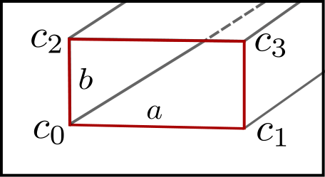
See also
The waveguide example shows a full waveguide inlet setup on a rectangular geometry.
Time Coupling Strategy#
The subsection time coupling strategy controls how often the
electromagnetic fields are recomputed during the time evolution of a coupled
(multiphysics) problem.
type: selects the coupling strategy:none(default): solved once before the first time step and never recomputed.iteration: recompute everycoupling iterationtime iterations.time: recompute everycoupling timeunits of physical time.threshold: recompute whenever the electromagnetic properties of the medium change by more thancoupling threshold.
coupling iteration: number of time iterations between two electromagnetic solves whentype = iteration.coupling time: physical time interval between two electromagnetic solves whentype = time.coupling threshold: the maximum change ratio across all electromagnetic properties of the medium \(\Delta_{\mathrm{properties}}> \mathrm{threshold}\) that triggers a new solve whentype = threshold. The computation of this ratio is given by the following formula:\[\Delta_{\mathrm{properties}} = \max_{K,q}\left(\frac{\left|\varepsilon_{r,\mathrm{eff}}^{\mathrm{current}}(\mathbf{x}_{K,q})-\varepsilon_{r,\mathrm{eff}}^{\mathrm{last}}(\mathbf{x}_{K,q})\right|}{\left|\varepsilon_{r,\mathrm{eff}}^{\mathrm{last}}(\mathbf{x}_{K,q})\right|},\frac{\left|\mu_{r}^{\mathrm{current}}(\mathbf{x}_{K,q})-\mu_{r}^{\mathrm{last}}(\mathbf{x}_{K,q})\right|}{\left|\mu_{r}^{\mathrm{last}}(\mathbf{x}_{K,q})\right|}\right)\]where \(K\) is the element index, \(q\) is the quadrature point index, and \(\mathbf{x}_{K,q}\) is the physical coordinate of the quadrature point. The superscripts
currentandlastrefer to the current and last time the electromagnetic fields were solved, respectively.