Gas-Solid Spouted Rectangular Bed

Features

• Solvers: lethe-particles and lethe-fluid-particles

• Three-dimensional problem

• Simulates a gas-solid spouted bed

• Compares the simulation results to experimental results

Files Used in This Example

The files mentioned below are located in the example’s folder (examples/unresolved-cfd-dem/gas-solid-spouted-rectangular-bed).

• Python functions script using Lagrangian post-processing: functions_lagrangian.py

• Python functions script using particles: functions_particles.py

• Parameter file for CFD-DEM simulation of the spouted bed: gas-solid-spouted-rectangular-bed.prm

• Parameter file for particle generation and packing: packing-particles.prm

• Python post-processing script using Lagrangian post-processing: postprocessing_lagrangian.py

• Python post-processing script using particles: postprocessing_particles.py

Description of the Case

This example simulates the spouting of spherical particles in air. The lethe-particles solver is used to fill the bed with particles, then the lethe-fluid-particles solver is used to simulate the spouting of the particles. Check-pointing is enabled in order to write the DEM checkpoint files to be used as the starting point of the CFD-DEM simulation. Using the parameters suggested by Geitani et al. [1], the simulation is run and the results are then compared to the experimental results from Yue et al. [2]

DEM Parameter File

All parameter subsections are described in the parameter section of the documentation.

To set-up the rectangular spouted bed case, the bed is filled with particles to obtain a static bed height of 200 mm.

The different subsections of the parameter file packing-particles.prm needed to run this simulation are introduced below.

Mesh

The following figure shows the geometry of the mesh:

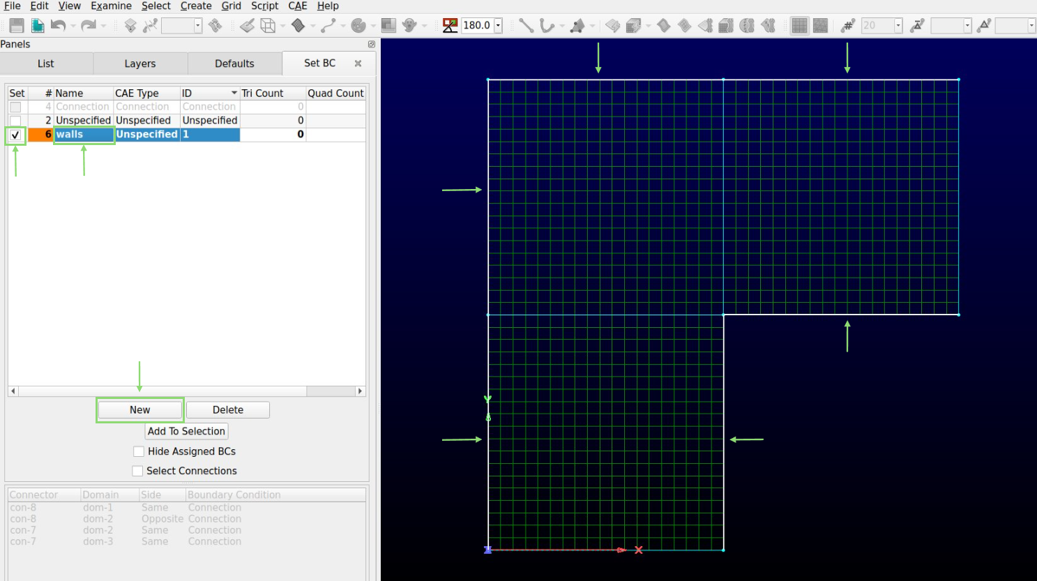
The dimensions shown in the figure are in millimeters, and the bed and the channel both have a depth of 40 mm. The flow is introduced through a channel that is connected to the bed. The geometry of the bed was created using GMSH. The mesh is created using the same dimensions as used by Geitani et al. [1] in order to compare the simulation results to the experimental results obtained by Yue et al. [2]. The mesh file is in the GMSH format and is located in the mesh folder.

subsection mesh
  set type                                = gmsh
  set file name                           = ./mesh/spouted_structured.msh
  set expand particle-wall contact search = false
end

Simulation Control

In the simulation control subsection, the time end is set to 1.5 s with a time step of 0.00001 s, which is long enough to allow the particles to come to rest. Additionally, users can specify the output folder for the simulation results in this subsection.

subsection simulation control
  set time step        = 0.00001
  set time end         = 1.5
  set log frequency    = 1000
  set output frequency = 10000
  set output path      = ./output_dem/
end

Restart

The lethe-fluid-particles solver requires reading several DEM files to start the simulation. The check-pointing option is enabled in the restart subsection.

subsection restart
  set checkpoint = true
  set frequency  = 10000
  set restart    = false
  set filename   = dem
end

Model Parameters

The following parameters are chosen for the model parameters subsection. Dynamic load balancing is enabled to achieve better computational performance.

subsection model parameters
  subsection contact detection
    set contact detection method                = dynamic
    set dynamic contact search size coefficient = 0.9
    set neighborhood threshold                  = 1.3
  end
  subsection load balancing
    set load balance method     = dynamic
    set threshold               = 0.5
    set dynamic check frequency = 10000
  end
  set particle particle contact force method = hertz_mindlin_limit_overlap
  set particle wall contact force method     = nonlinear
  set integration method                     = velocity_verlet
end

Lagrangian Physical Properties

The gravitational acceleration as well as the physical properties of the particles and the walls are specified in the lagrangian physical properties subsection. In order to obtain a static bed height of 200 mm, 175800 spherical particles with a diameter of 2.5 mm are inserted into the rectangular bed. All of the particle properties defined in this subsection are the same as those used by Geitani et al. [1]

subsection lagrangian physical properties
  set g                        = 0.0, -9.81, 0.0
  set number of particle types = 1
  subsection particle type 0
    set size distribution type            = uniform
    set diameter                          = 0.0025
    set number                            = 175800
    set density particles                 = 2500
    set young modulus particles           = 1e7
    set poisson ratio particles           = 0.25
    set restitution coefficient particles = 0.9
    set friction coefficient particles    = 0.3
    set rolling friction particles        = 0
  end
  set young modulus wall           = 1e7
  set poisson ratio wall           = 0.25
  set restitution coefficient wall = 0.9
  set friction coefficient wall    = 0.3
  set rolling friction wall        = 0
end

Insertion Info

The insertion info subsection manages the insertion of particles. The volume of the insertion box is large enough to fit all the particles. The insertion info parameters are set in order to avoid particle collisions during the packing process.

subsection insertion info
  set insertion method                               = volume
  set inserted number of particles at each time step = 43950
  set insertion frequency                            = 30000
  set insertion box points coordinates               = -0.139, 0.3, 0.001 : 0.139, 0.525, 0.039
  set insertion distance threshold                   = 1.5
  set insertion maximum offset                       = 0.3
  set insertion prn seed                             = 19
end

Floating Walls

A floating wall is used to prevent the particles from falling into the inlet channel. Its position is shown in the figure in the mesh subsection. The floating wall is defined at the top of the channel, which is at a y-coordinate of 0, and is set to remain active for the entire simulation time.

subsection floating walls
  set number of floating walls = 1
  subsection wall 0
    subsection point on wall
      set x = 0
      set y = 0
      set z = 0
    end
    subsection normal vector
      set nx = 0
      set ny = 1
      set nz = 0
    end
    set start time = 0
    set end time   = 50
  end
end

Running the DEM Simulation

Assuming that the lethe-particles executable is within your path, the simulation can be launched in parallel using the following command:

mpirun -np 10 lethe-particles packing-particles.prm

Note

Running the packing should take approximately 45 minutes on 10 cores.

After the particles have been packed inside the rectangular bed, it is now possible to simulate the spouting of the particles.

CFD-DEM Parameter File

The CFD-DEM simulation is to be carried out using the packed bed simulated in the previous step.

Simulation Control

The simulation is run for 10 s with a time step of 0.0005 s. The time scheme chosen for the simulation is second order backward differentiation method (BDF2).

subsection simulation control
  set method               = bdf2
  set output frequency     = 50
  set time end             = 10
  set time step            = 0.0005
  set subdivision          = 1
  set log precision        = 10
  set output path          = ./output/
end

Physical Properties

A density of 1 and a kinematic viscosity of 0.0000181 are defined in the physical properties subsection to simulate the flow of air.

subsection physical properties
  subsection fluid 0
    set kinematic viscosity = 0.0000181
    set density             = 1
  end
end

Initial Conditions

A zero velocity field is used as the initial condition.

subsection initial conditions
  subsection uvwp
      set Function expression = 0; 0; 0; 0
  end
end

Boundary Conditions

The figure presented in the mesh subsection of this example shows the corresponding boundary IDs for each outer surface. A slip boundary condition is applied on all the walls of the bed and the channel (ID 0 and ID 3), except the inlet at the bottom of the channel (ID 1) and the outlet on the top of the bed (ID 2).

At the base of the channel, a time dependent Dirichlet boundary condition is imposed. To avoid an initial shock from the introduction of high velocity gas in the bed, the inlet is linearly velocity is increased from 0 m/s at t = 0 s until it reaches 20.8 m/s at t = 0.05 s.

subsection boundary conditions
  set time dependent = true
  set number         = 4
  subsection bc 0
    set id   = 0
    set type = slip
  end
  subsection bc 1
    set id   = 1
    set type = function
    subsection u
      set Function expression = 0
    end
    subsection v
      set Function expression = if(t<0.05,416*t,20.8)
    end
    subsection w
      set Function expression = 0
    end
  end
  subsection bc 2
    set id   = 2
    set type = outlet
  end
  subsection bc 3
    set id   = 3
    set type = slip
  end
end

The additional sections for the CFD-DEM simulations are the void fraction subsection and the CFD-DEM subsection. These subsections are described in detail in the CFD-DEM parameters .

Void Fraction

Since the void fraction is calculated using the packed bed of the DEM simulation, the mode is set to dem. To read the dem files, read dem is set to true and the prefix of the dem files is specified. The quadrature centered method (QCM) is chosen to calculate the void fraction.

subsection void fraction
  set mode                         = qcm
  set read dem                     = true
  set dem file name                = dem
  set l2 smoothing length          = 0.0075
  set particle refinement factor   = 0
end

CFD-DEM

In the cfd-dem subsection, grad-div stabilization is enabled to improve local mass conservation, and the void fraction time derivative is enabled to account for the time variation of the void fraction.

subsection cfd-dem
  set grad div                      = true
  set void fraction time derivative = true
  set drag force                    = true
  set buoyancy force                = true
  set shear force                   = true
  set pressure force                = true
  set saffman lift force            = false
  set drag model                    = difelice
  set coupling frequency            = 100
  set implicit stabilization        = false
  set grad-div length scale         = 0.1
  set vans model                    = modelA
end

Non-linear Solver

The inexact_newton solver is used to avoid the reconstruction of the system matrix at each Newton iteration. For more information about the non-linear solver, please refer to the Non-Linear Solver Section

subsection non-linear solver
  subsection fluid dynamics
    set solver           = inexact_newton
    set tolerance        = 1e-6
    set max iterations   = 25
    set verbosity        = verbose
    set matrix tolerance = 0.8
  end
end

Linear Solver

The linear solver is defined according to the parameters suggested by Geitani et al. [1] The absolute tolerance for the linear solver is set to a value 100 times smaller than the tolerance of the non-linear solver to ensure the non-linear solver converges.

subsection linear solver
  subsection fluid dynamics
    set method                                = gmres
    set max iters                             = 200
    set relative residual                     = 1e-4
    set minimum residual                      = 1e-8
    set preconditioner                        = ilu
    set ilu preconditioner fill               = 1
    set ilu preconditioner absolute tolerance = 1e-10
    set ilu preconditioner relative tolerance = 1
    set verbosity                             = verbose
    set max krylov vectors                    = 200
  end
end

Running the CFD-DEM Simulation

Assuming that the lethe-fluid-particles executable is within your path, the simulation can be launched using the following command:

mpirun -np 10 lethe-fluid-particles gas-solid-spouted-rectangular-bed.prm

Note

Running the CFD-DEM simulation should take approximately 1.5 days on 10 cores.

Post-processing

It is possible to run the post-processing code to post-process the particle velocities with the following line, with the simulation path as the argument:

  python3 postprocessing_particles.py  --folder ./

The functions used in the post-processing script are defined in the functions-particles.py file. This post-processing script reads the particle velocity data and plots the particle velocities as a function of the x-position in the bed for different y-heights.

It is also possible to run the post-processing code using the lagrangian post-processing output with the following line, with the simulation path as the argument:

  python3 postprocessing_lagrangian.py  --folder ./

The functions used in the post-processing script are defined in the functions-lagrangian.py file. This post-processing script uses the average particle velocities at each mesh point to plot the particle velocities as a function of the x-position in the bed for different y-heights.

For more information about the Lagrangian post-processing, please refer to the Post-processing Section.

Important

You need to ensure that lethe_pyvista_tools is working on your machine. Click here for details.

Results and Discussion

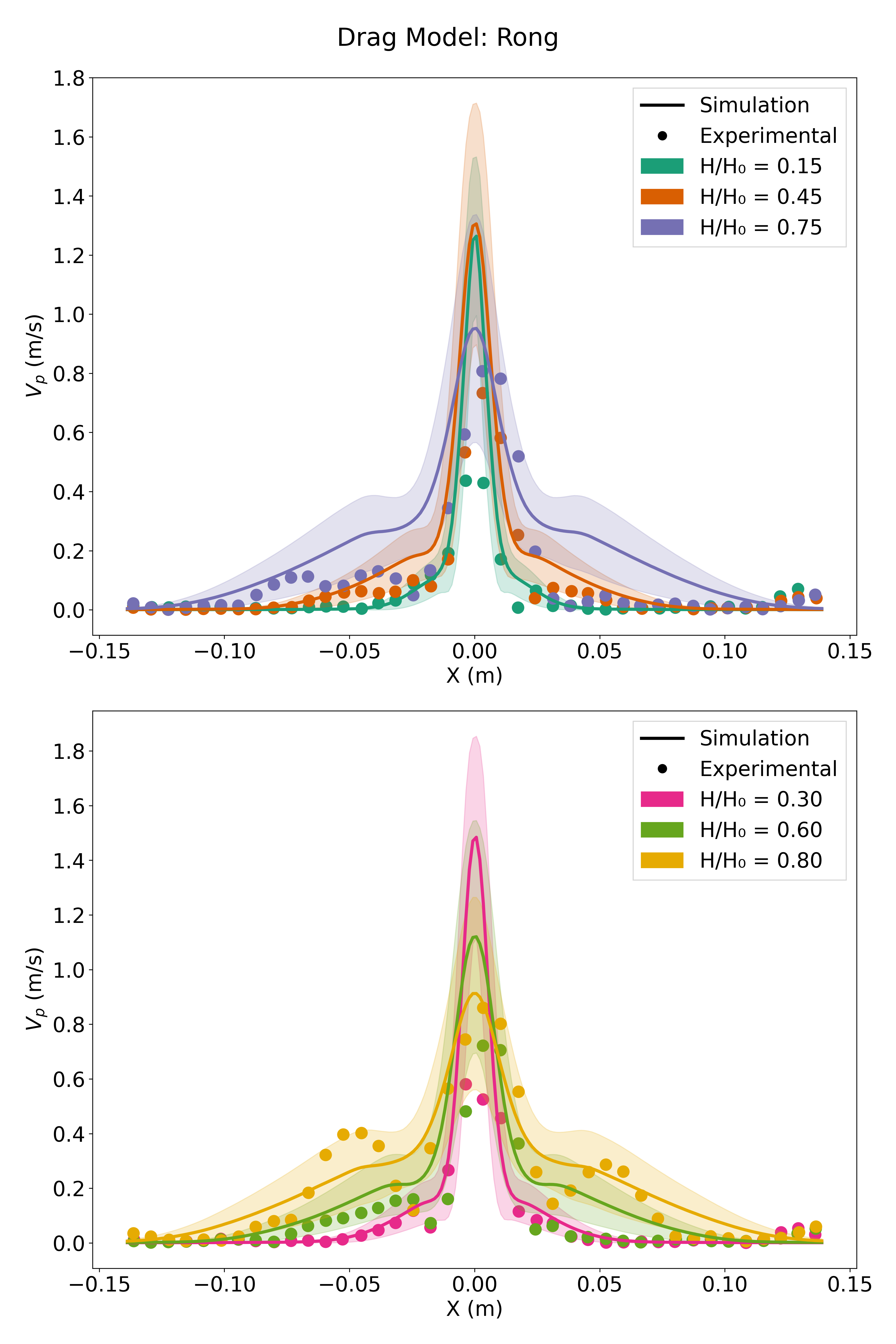
Using the postprocessing_particles.py post-processing script, the particle velocity magnitudes are plotted, in the following figure, as a function of the x-position in the bed, for different y-heights. The simulation is run with the Rong drag model to compare the results with the results obtained with the Di Felice drag model.

The experimental results from Yue et al. [2] are shown in the same figure for comparison. The standard deviation of the particle velocity magnitudes is shown as a shaded area around the average velocity magnitude. The two drag models lead to different results mainly at the center of the bed, where the spouting occurs, with the Rong drag model leading to higher particle velocity magnitudes than the Di Felice drag model. The particle velocity magnitudes are in good agreement with the experimental results, especially at the center of the bed, where the spouting occurs.

The following animation shows the spouting of the particles as the gas is introduced from the channel at the base of the bed. The void fraction profile is shown as well.

References

[1] (1,2,3,4)

T. E. Geitani, S. Golshan, and B. Blais, “Toward High-Order CFD-DEM: Development and Validation,” Industrial & Engineering Chemistry Research, vol. 62, no. 2, pp. 1141-1159, Jan. 2023, doi: 10.1021/acs.iecr.2c03546.

[2] (1,2,3)

Y. Yue, S. Wang, P. Bahl, C. de Silva, and Y. Shen, “Experimental Investigation of Spout Deflection in a Rectangular Spouted Bed by the PIV Method,” Industrial & Engineering Chemistry Research, vol. 59, no. 30, pp. 13810-13819, Jun. 2020, doi: 10.1021/acs.iecr.0c02060.