Boycott Effect#
Features#
Solvers:
lethe-particlesandlethe-fluid-particlesThree-dimensional problem
Displays the selection of models and physical properties
Simulates a solid-liquid sedimentation
Files Used in This Example#
Both files mentioned below are located in the example’s folder (examples/unresolved-cfd-dem/boycott-effect).
Parameter file for initial particles generation:
initial-particles.prmParameter file for CFD-DEM simulation of the Boycott effect:
boycott-effect.prm
Description of the Case#
This example simulates the sedimentation of a group of particles in a viscous fluid. Two cases were simulated. In the first case, the channel is placed vertically. In the second case, the channel is inclined at \(20^{\circ}\) with respect to the gravity. First, we use lethe-particles to insert the particles. We enable check-pointing in order to write the DEM checkpoint files which will be used as the starting point of the CFD-DEM simulation. Then, we use the lethe-fluid-particles solver within Lethe to simulate the sedimentation of particles by initially reading the checkpoint files from the DEM simulation.
DEM Parameter File#
We introduce the different sections of the parameter file boycott-effect.prm needed to run this simulation. Most subsections are explained in detail in other CFD-DEM examples such as: Gas-solid spouted bed. Therefore, we will not go over them in detail.
Mesh#
In this example, we are simulating a rectangular channel. We use the deal.II GridGenerator in order to generate a hyper rectangle that is subdivided along its height. The following portion of the DEM parameter file shows the function called:
subsection mesh
  set type                                = dealii
  set grid type                           = subdivided_hyper_rectangle
  set grid arguments                      = 15,70,15:-0.03,0,-0.03:0.03,0.4,0.03:true
  set initial refinement                  = 0
  set expand particle-wall contact search = false
end
Simulation Control#
The time step in this case is the same as the time end. Since we only seek to insert the particles at the top of the channel, we only require 1 insertion time step. We do not need the particles to be packed, therefore by doing this, the particles will be inserted, but will not fall under the action of gravity.
subsection simulation control
   set time step        = 1e-6
   set time end         = 1e-6
   set log frequency    = 1000
   set output frequency = 1
   set output path      = ./output_dem/
 end
Restart#
We save the files obtained from the single iteration by setting the frequency = 1. These files will be used to start the CFD-DEM simulation.
subsection restart
  set checkpoint = true
  set frequency  = 1
  set restart    = false
  set filename   = dem
end
Model Parameters#
The section on model parameters is explained in the DEM examples. We show the chosen parameters for this section:
subsection model parameters
  subsection contact detection
    set contact detection method = dynamic
    set neighborhood threshold   = 1.3
    set frequency                = 1
  end
  set rolling resistance torque method       = constant
  set particle particle contact force method = hertz_mindlin_limit_force
  set particle wall contact force method     = nonlinear
  set integration method                     = velocity_verlet
end
Lagrangian Physical Properties#
The gravity is set to 0 as we only need to insert the particles in the specified insertion box.
subsection lagrangian physical properties
  set g                        = 0.0, 0.0, 0.0
  set number of particle types = 1
  subsection particle type 0
    set size distribution type            = uniform
    set diameter                          = 0.002
    set number                            = 8379
    set density particles                 = 1200
    set young modulus particles           = 1e6
    set poisson ratio particles           = 0.25
    set restitution coefficient particles = 0.97
    set friction coefficient particles    = 0.3
    set rolling friction particles        = 0.1
  end
  set young modulus wall           = 1e6
  set poisson ratio wall           = 0.25
  set restitution coefficient wall = 0.97
  set friction coefficient wall    = 0.3
  set rolling friction wall        = 0.1
end
Insertion Info#
We insert the particles uniformly in the specified insertion box at the top of the channel.
subsection insertion info
  set insertion method                               = volume
  set inserted number of particles at each time step = 8379
  set insertion frequency                            = 2000
  set insertion box points coordinates               = -0.025, 0.3, -0.025 : 0.026, 0.396, 0.026
  set insertion distance threshold                   = 1.2
  set insertion maximum offset                       = 0.
  set insertion prn seed                             = 19
end
Running the DEM Simulation#
Launching the simulation is as simple as specifying the executable name and the parameter file. Assuming that the lethe-particles executable is within your path, the simulation can be launched on a single processor by typing:
or in parallel (where 8 represents the number of processors)
The figure below shows the particles inserted at the top of the channel at the end of the DEM simulation.
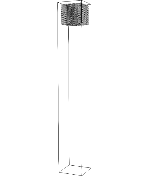
After the particles have been inserted it is now possible to simulate the sedimentation of particles.
CFD-DEM Parameter File#
The CFD simulation is to be carried out using the particles inserted within the previous step. We will discuss the different parameter file sections. Some sections are identical to that of the DEM so they will not be shown again.
Simulation Control#
The simulation is run for \(2\) s with a time step of \(0.005\) s. The time scheme chosen for the simulation is first order backward difference method (BDF1). The simulation control section is shown:
subsection simulation control
  set method               = bdf1
  set number mesh adapt    = 0
  set output name          = result_
  set output frequency     = 20
  set time end             = 2
  set time step            = 0.005
  set output path          = ./output/
end
Physical Properties#
The physical properties subsection allows us to determine the density and viscosity of the fluid. We choose a density of \(1115.6\) and a kinematic viscosity of \(0.00000177\) as to simulate the flow of a sugar-water solution with \(20\) % by weight sugar at \(20^{\circ}\) C. The dynamic viscosity of a 20 % sugar-water solution by weight at \(20^{\circ} C\) is 1.97 cP.
subsection physical properties
  subsection fluid 0
    set kinematic viscosity = 0.00000177
    set density             = 1115.6
  end
end
Initial Conditions#
For the initial conditions, we choose zero initial conditions for the velocity.
subsection initial conditions
  set type = nodal
  subsection uvwp
    set Function expression = 0; 0; 0; 0
  end
end
Boundary Conditions#
For the boundary conditions, we choose a slip boundary condition on all the walls of the channel and the channel except the bottom and the top of the channel where a no-slip boundary condition is imposed. For more information about the boundary conditions, please refer to the Boundary Conditions Section
subsection boundary conditions
  set number = 6
  subsection bc 0
    set id   = 0
    set type = slip
  end
  subsection bc 1
    set id   = 1
    set type = slip
  end
  subsection bc 2
    set id   = 2
    set type = noslip
  end
  subsection bc 3
    set id   = 3
    set type = noslip
  end
  subsection bc 4
    set id   = 4
    set type = slip
  end
  subsection bc 5
    set id   = 5
    set type = slip
  end
end
Lagrangian Physical Properties#
This section is identical to the one previously mentioned for the DEM simulation of particle insertion. The only difference is the definition of gravity. For the vertical case, we set \(g_y = -9.81\) and \(g_x = g_z = 0\). For the inclined case, we determine the gravity by setting: \(g_x = \frac{-9.81}{cos \theta}, \; g_y = \frac{-9.81}{sin \theta}, \; g_z = 0\) where \(\theta\) is the angle of inclination with the vertical.
The additional sections for the CFD-DEM simulations are the void fraction subsection and the CFD-DEM subsection. These subsections are descrichannel in detail in the CFD-DEM parameters .
Void Fraction#
Since we are calculating the void fraction using the particle insertion of the DEM simulation, we set the mode to dem. For this, we need to read the dem files which we already wrote using check-pointing. We, therefore, set the read dem to true and specify the prefix of the dem files to be dem.
We choose to use the quadrature centered method (QCM) to calculate the void fraction. For this, we specify the mode to be qcm. We want the radius of our volume averaging sphere to be equal to the length of the element where the void fraction is being calculated. We don’t want the volume of the sphere to be equal to the volume of the element.
For this, we set the qcm sphere equal cell volume equals to false. Unlike the other schemes, we do not smooth the void fraction as we usually do using the PCM and SPM void fraction schemes since QCM is continuous in time and space.
subsection void fraction
  set mode                         = qcm
  set qcm sphere equal cell volume = false
  set read dem                     = true
  set dem file name                = dem
end
CFD-DEM#
We also enable grad-div stabilization in order to improve local mass conservation. If we were using PCM and SPM void fraction schemes, the void fraction time derivative should be disabled as the time variation of the void fraction will lead to unstable simulations. The source of such instability is the first term of the continuity equation \(\rho_f \frac{\partial \varepsilon_f}{\partial t}\), which is stiff and unstable for the slightest temporal discontinuity of the void fraction and as \(\Delta t \to 0\). However, as we are using the QCM void fraction scheme, this term can be enabled. Usually, this term is neglected, however; disabling this term affects the results as we are no longer solving for the actual Volume Averaged Navier-Stokes equations. Therefore, we should not neglect this term based on numerical reasoning without any physical explanation.
subsection cfd-dem
  set grad div                      = true
  set void fraction time derivative = true
  set drag force                    = true
  set buoyancy force                = true
  set shear force                   = true
  set pressure force                = true
  set drag model                    = difelice
  set coupling frequency            = 250
  set grad-div length scale         = 0.005
  set vans model                    = modelA
end
We determine the drag model to be used for the calculation of particle-fluid forces. We enable buoyancy, drag, shear and pressure forces. For drag, we use the Di Felice model to determine the momentum transfer exchange coefficient. The VANS model we are solving is model A. Other possible option is model B.
Finally, the linear and non-linear solver controls are defined.
Non-linear Solver#
subsection non-linear solver
  subsection fluid dynamics
    set solver           = inexact_newton
    set tolerance        = 1e-8
    set max iterations   = 10
    set verbosity        = verbose
    set matrix tolerance = 0.75
  end
end
We use the inexact_newton solver as to avoid the reconstruction of the system matrix at each Newton iteration. For more information about the non-linear solver, please refer to the Non Linear Solver Section
Linear Solver#
subsection linear solver
  subsection fluid dynamics
    set method                                = gmres
    set max iters                             = 5000
    set relative residual                     = 1e-3
    set minimum residual                      = 1e-10
    set preconditioner                        = ilu
    set ilu preconditioner fill               = 0
    set ilu preconditioner absolute tolerance = 1e-12
    set ilu preconditioner relative tolerance = 1
    set verbosity                             = verbose
    set max krylov vectors                    = 200
  end
end
For more information about the linear solver, please refer to the Linear Solver Section
Running the CFD-DEM Simulation#
The simulation is run using the lethe-fluid-particles application. Assuming that the executable is within your path, the simulation can be launched as per the following command:
Results#
The results are shown in an animation below. The sedimentation of the particles in a vertical and inclined channel demonstrate different behaviors. This clearly shows the boycott effect as the fluid circulates in the inclined channel resulting in a larger velocity for both the fluid and particles. Thus, the particles fall further compared to the vertical channel where the fluid velocity is almost null, and the particles’ acceleration is low.