Paddle Mixer Using the Mortar Method#
This example showcases the use of the mortar method in Lethe to solve a 2D incompressible flow problem with a rotating impeller.
Features#
Solver:
lethe-fluid(with Q1-Q1)Transient problem
Mortar method for rotating geometry
Usage of gmsh files with mortar method
Files Used in This Example#
All files mentioned below are located in the example’s folder (examples/incompressible-flow/2d-paddle-mixer-mortar).
Geometry file:
full-geometry.stepRotor mesh file:
mixer_rotor.mshStator mesh file:
mixer_stator.mshParameter file:
paddle_mixer_mortar.prm
Description of the Case#
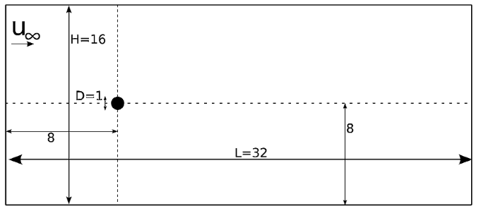
We simulate the flow around a rotating impeller in a cylindrical domain with the presence of a baffle. This domain is composed of the rotor part, which contains the impeller and is rotating, and the stationary stator part. These two geometries are attached with mortar elements, which maintain the continuity of the solution between the two domains.
The geometry of the problem is illustrated in the following figure:
Parameter File#
Simulation Control#
A 1st order backward differentiation is used for the time integration (bdf1), considering a 0.01 second time step and a final simulation time of 10 seconds. Outputs are saved every 5 steps, as indicated by the output frequency parameter.
subsection simulation control
  set method           = bdf1
  set time step        = 0.01
  set time end         = 10
  set output frequency = 5
  set output path      = ./output/
  set output name      = mortar-output
end
FEM#
For this example, Q1 elements are used for both velocity and pressure. The bubble enrichment function is also enabled for the velocity field to increase the accuracy and stability of the solution. The deal.II documentation contains more information about this enrichment function.
subsection FEM
  set enable bubble function velocity = true
  set velocity degree                  = 1
  set pressure degree                  = 1
end
Mesh#
When using the mortar method, only the static mesh needs to be included in the mesh subsection. In this example, mixer_stator.msh only contains the meshed stator shown in the above case description.
subsection mesh
  set type               = gmsh
  set file name          = mixer_stator.msh
  set initial refinement = 2
end
Mortar#
The mortar subsection specifies all the parameters required to simulate a rotor-stator geometry using mortar elements to attach the two meshes. The mesh subsection embedded in the mortar subsection refers to the rotor domain and contains the same parameters described in Mesh. Due to the current implementation, it is important that the number of cells on both sides of the mortar interface, as well as the angular length of these cells, are equal. The interface discretizations must also be geometrically aligned, which means each cell has a one-to-one match with aligned vertices on the other side. Different amount of cells on both sides or misalignment will fail the mortar cells generation step.
After the rotor geometry configuration, the boundary ids at the rotor-stator interface need to be specified. Other parameters related to the rotation of the rotor domain can also be modified (see the Mortar section for more details):
The
center of rotationrepresents the coordinates around which the rotor domain will be rotating.The
rotor rotation anglesubsection contains the expression for the rotation angle, which can either be constant or time-dependent.The
rotor angular velocitysubsection contains the expression for the angular velocity of the rotor and needs to correspond to the time derivative of therotor rotation angle.
We can now set verbosity to verbose to print information about the rotor rotation at every iteration. Lastly, we set the radius tolerance to 1e-6; every iteration, the radial distance between the center of rotation and every node at the rotor-stator interface is calculated to ensure that the difference between the maximum and minimum value is less than the tolerance. If this value exceeds the tolerance, the simulation will stop and an error message will be printed. This constraint serves as a sanity check : theoretically, all nodes at the rotor-stator interface should be at the same distance from the center of rotation. This check could fail for multiple reasons, such as a missing manifold setup for the circular interface, a misassignment of the mortar boundary ids or an insufficient precision in the mesh file.
Note
When creating the .msh files from the .step files, the boundary ids need to be unique for the rotor and stator domains. For example, if the boundary id for the rotor-stator interface is 3 in the rotor mesh, it should be 4 in the stator mesh. This way, both boundaries can be specified in the mortar subsection without any conflict. As of today, a manual modification of the .msh files may be required to achieve this. It is important to note that the boundary ids for the rotor and stator interface do not need to be sequential, as the only requirement is that they are unique.
subsection mortar
  set enable = true
  subsection mesh
    set type               = gmsh
    set file name          = mixer_rotor.msh
  end
  set rotor boundary id  = 3
  set stator boundary id = 4
  set center of rotation = 0, 0
  subsection rotor rotation angle
    set Function expression = 1*t
  end
  subsection rotor angular velocity
    set Function expression = 1
  end
  set verbosity = verbose
  set radius tolerance = 1e-6
end
Boundary Conditions#
Both the outside wall (ID 5) and the baffle (ID 6) have a no-slip Dirichlet boundary condition. The mortar boundaries (ID 3 and 4) are already defined in the mortar subsection, so a none boundary condition is assigned to them here. Finally, the velocity of the fluid at the impeller (ID 2) is defined with the functions \(u=-\omega y\) and \(v=\omega x\), where \(\omega\) is the angular velocity of the impeller, defined as 1 in the mortar subsection.
subsection boundary conditions
  set number = 3
  subsection bc 0
    set type               = noslip
    set id                 = 5,6
  end
  subsection bc 1
    set type               = none
    set id                 = 3,4
  end
  subsection bc 2
    set type = function
    set id   = 2
    subsection u
      set Function expression = -y
    end
    subsection v
      set Function expression = x
    end
  end
end
Manifolds#
Since the mortar boundary and the outside wall are both circular, we need to setup manifolds to ensure that the circular shape is not lost as the mesh is refined. See the Manifolds section for more information about the manifold types supported in Lethe.
subsection manifolds
  set number = 3
  subsection manifold 0
    set id = 3
    set type = spherical
    set point coordinates = 0, 0
  end
  subsection manifold 1
    set id = 4
    set type = spherical
    set point coordinates = 0, 0
  end
  subsection manifold 2
    set id = 5
    set type = spherical
    set point coordinates = 0, 0
  end
end
Linear Solver#
The only modification made in the linear solver is the use of the AMG preconditioner.
subsection linear solver
  subsection fluid dynamics
    set verbosity                             = quiet
    set method                                = gmres
    set preconditioner                        = amg
  end
end
Running the Simulation#
Assuming that the lethe-fluid executable is within your path, the simulation can be launched in parallel using MPI by typing:
with X the number of processors used to run it. The simulation is not extensively long; it takes approximately 8 minutes on 1 core of a AMD Ryzen 9 5900X 12-Core Processor.
Lethe will generate a number of files. The most important one bears the extension .pvd. It can be read by visualization programs such as Paraview.
Results and Discussion#
Using Paraview, we can visualize the results of the simulation with the .pvd output file. Using the surface LIC visualization method, we obtain the following animation:
As we can see, the presence of the baffle creates re-circulation zones in the flow, which are visible in the animations. Continuity of the solution is maintained at the mortar interface, as expected.
Possibilities for Extension#
Vary the Reynolds number to see the effect on the flow.
Run the simulation for different impeller and/or baffle geometries.
Make the case three-dimensional by using a cylindrical mortar interface.