Capillary Wave

This example simulates the damping of a small amplitude capillary wave for different time-steps allowing us to study the capillary time-step constraint. The problem is inspired by the test case of Denner et al. [1]

Features

• Solver: lethe-fluid

• Volume of fluid (VOF)

• Unsteady problem handled by an adaptive BDF2 time-stepping scheme

• Bash scripts to write, launch, and postprocess multiple cases

• Python scripts for postprocessing data

Files Used in This Example

All files mentioned below are located in the example’s folder (examples/multiphysics/capillary-wave).

• Analytical data: capillaryWaveData_rho_1_nu_5e-6_prosperetti.csv

• Analytical solution computation Python script: capillary-wave-prosperetti-solution.py

• Case generation and simulation launching Bash script: capillary-wave-time-step-sensitivity.sh

• Parameter file for case generation: capillary-wave.tpl

• Parameter file for the \(\Delta t = 0.95\Delta t_\sigma\) case: capillary-wave-TSM-0_95.prm

• Postprocessing Python script for a simple case: capillary-wave-postprocess.py

• Postprocessing Python script for generating a comparison figure: capillary-wave-combined.py

• Postprocessing Bash script: capillary-wave-time-step-sensitivity-postprocess.sh

• Python script for computing quantities of interest: capillary-wave-calculation.py

Description of the Case

Have you ever tried skipping stones on a pond or at the beach? If so, you have likely observed the mesmerizing ripples that form when the stone makes contact with the water’s surface. Ripples and waves are an integral part of our everyday lives. You can witness their presence at the beach, where surfers ride them, when swimming in a swimming pool, or even when you drop a cube of sugar into your morning coffee. Notably, these phenomena occur at different length scales and propagate at a velocity (\(c\)), often referred to as the phase velocity. Under the assumption that viscous stresses are negligible, the phase velocity of a single wave can be expressed as follows:

\[c = \frac{\omega}{k}=\frac{\omega\lambda}{2\pi}=\sqrt{\frac{(\rho_1-\rho_0)g\lambda}{\hat{\rho}2\pi} + \frac{2\pi\sigma}{\hat{\rho}\lambda}}\]

where \(\omega=\sqrt{\frac{\rho_1-\rho_0}{\hat{\rho}}gk+\frac{\sigma k^3}{\hat{\rho}}}\) is the angular frequency of the wave with, \(\sigma\), the surface tension coefficient, \(k=\frac{2\pi}{\lambda}\) is the wavenumber with, \(\lambda\), the wavelength, \(g\) is the gravitational acceleration, and \(\hat{\rho} = \rho_0 + \rho_1\) is the sum of the densities of the fluids [2, 3].

The first term beneath the square root accounts for the gravitational contribution, while the second term is a result of surface tension. Depending on the wavelength, either of these contributions may dominate the other. When:

• \(\lambda \gg 2\pi l_\sigma\), gravity dominates surface tension and we get what we call a gravity wave (see Sloshing in a Rectangular Tank).

• \(\lambda \ll 2\pi l_\sigma\), surface tension dominates gravity and we get a capillary wave.

\(l_\sigma=\sqrt{\frac{\sigma}{\rho g}}\) is the capillary length.

In this example, we simulate the damping of a small amplitude capillary wave in a rectangular domain of dimensions \(\lambda \times 3\lambda\) with \(\lambda=10^{-4}\). The selected initial amplitude of the wave is \(a_0=0.01\lambda\) giving us the following expression for the initial height of the wave:

\[y_0(x) = a_0 \cos\left( \frac{2\pi}{\lambda} x \right) = 1 \times 10^{-6} \cos\left(2\times 10^{-4}\pi x \right)\]

Note

The origin of the plane \(\left( (x,y)=(0,0) \right)\) is located at the center of the domain.

Initial state of the wave

Neglecting the gravitational contribution, the phase velocity of the wave may be expressed as:

\[c_\sigma = \sqrt{\frac{2\pi\sigma}{\hat{\rho}\lambda_\sigma}}\]

and the angular frequency simply becomes:

\[\omega_\sigma = \sqrt{\frac{\sigma}{\hat{\rho}} \left(\frac{2\pi}{\lambda_\sigma}\right)^3}\]

Since, the phase fraction (\(\phi\)) is treated explicitly, the temporal resolution of the capillary wave leads to a Courant-Friedrichs-Lewy (CFL) condition, also known as the capillary time-step constraint:

\[\Delta t_\sigma = \frac{\Delta x}{\sqrt{2} c_\sigma} = \sqrt{\frac{\hat{\rho}}{2\pi\sigma}{{\Delta x}^3}}\]

with the shortest unambiguously resolved capillary wave having a wavelength of \(\lambda_\sigma = 2 \Delta x\) [2].

Therefore, in order to get stable simulation results, \(\Delta t < \Delta t_\sigma\) should be respected. In this example, different time-steps will be used to explore the stability limit of Lethe’s current implementation.

Parameter File

Simulation Control

Below, the simulation control subsection for the case of \(\Delta t \approx 0.95\Delta t_\sigma \approx 0.95(3.9 \times 10^{-9})\, \text{s}\) is shown. For other cases, the time step value will change and accordingly the output frequency will also.

The time integration is handled by a 2nd-order backward differentiation scheme (bdf2) with a constant time-step of \(\Delta t=3.7 \times 10^{-9} \, \text{s}\). To assess the stability of the simulation results, the wave is simulated for \(t_{\text{end}} = \frac{50}{\omega_\sigma} \approx 4.5 \times 10^{-5} \, \text{s}\).

subsection simulation control
  set method           = bdf2
  set time end         = 0.000045
  set time step        = .0000000037
  set output name      = capillary-wave-TSM-0_95
  set output frequency = 243
  set output path      = ./output-TSM-0_95/
end

Multiphysics

The multiphysics subsection is used to enable the VOF solver.

subsection multiphysics
  set VOF  = true
end

Initial Conditions

In the initial conditions, we define the initial height of the wave, such that the interface (\(\phi = 0.5\) isocurve) lies at the right height.

subsection initial conditions
  set type = nodal
  subsection uvwp
    set Function expression = 0; 0; 0
  end
  subsection VOF
    set Function expression = if (y<=1e-6*cos(2*3.14159/1e-4*x), min(0.5-(y-1e-6*cos(2*3.14159/1e-4*x))/1e-6,1), max(0.5-(y-1e-6*cos(2*3.14159/1e-4*x))/1e-6,0))
    subsection projection step
      set enable           = true
      set diffusion factor = 1
    end
  end
end

Mesh

In the mesh subsection, we define a subdivided hyper rectangle with appropriate dimensions. The mesh is initially refined \(4\) times to ensure adequate definition of the interface.

subsection mesh
  set type               = dealii
  set grid type          = subdivided_hyper_rectangle
  set grid arguments     = 4, 12 : -5e-5, -1.5e-4 : 5e-5, 1.5e-4 : true
  set initial refinement = 4
end

Mesh Adaptation

In the mesh adaptation subsection, we dynamically adapt the mesh using the phase as refinement variable. We choose \(3\) as the min refinement level and \(5\) as the max refinement level. We set initial refinement steps = 4 to adapt the mesh to the initial value of the VOF field.

subsection mesh adaptation
  set type                     = kelly
  set variable                 = phase
  set fraction type            = fraction
  set max refinement level     = 5
  set min refinement level     = 3
  set frequency                = 1
  set fraction refinement      = 0.95
  set fraction coarsening      = 0.05
  set initial refinement steps = 4
end

Physical Properties

In the physical properties subsection, we define the fluids such that both fluids have the same properties. We set the density to \(1\) and the kinematic viscosity to \(5 \times 10^{-6}\). A fluid-fluid type of material interaction is also defined to specify the surface tension model. In this case, it is set to constant with the surface tension coefficient set to \(0.01\).

subsection physical properties
  set number of fluids = 2
  subsection fluid 1
    set density             = 1
    set kinematic viscosity = 5e-6
  end
  subsection fluid 0
    set density             = 1
    set kinematic viscosity = 5e-6
  end
  set number of material interactions = 1
  subsection material interaction 0
    set type = fluid-fluid
    subsection fluid-fluid interaction
      set first fluid id              = 0
      set second fluid id             = 1
      set surface tension model       = constant
      set surface tension coefficient = 0.01
    end
  end
end

Running the Simulation

We can call lethe-fluid for each time step value. For \(\Delta t \approx 0.95\Delta t_\sigma\), this can be done by invoking the following command:

mpirun -np 4 lethe-fluid capillary-wave-TSM-0_95.prm

to run the simulation using four CPU cores. Feel free to use more CPU cores.

Warning

Make sure to compile Lethe in Release mode and run in parallel using mpirun. This simulation takes \(\sim \, 35\) minutes for \(\Delta t\approx 0.95\Delta t_\sigma\) and decreases to \(\sim \, 3\) minutes for \(\Delta t\approx 20\Delta t_\sigma\) on \(4\) processes.

Tip

In order to calculate the capillary time-step constraint and the simulation end time, a small Python script is provided, you may run it using:

python3 capillary-wave-calculation.py calculations.output

with calculations.output being the file where the results will be saved. If you omit this argument, results will simply be displayed in the terminal window.

Attention

The number of refinements (n_refinement) that you enter on line \(67\) of the script should correspond to the finest level of refinement of the mesh. In other words, it should correspond to the max refinement level of the mesh adaptation subsection of the parameter file.

n_refinement = 5 # Make sure that this value corresponds to the finest refinement level of your simulation

Tip

If you want to generate and launch multiple cases consecutively, a Bash script (capillary-wave-time-step-sensitivity.sh) is provided. Make sure that the file has executable permissions before calling it with:

./capillary-wave-time-step-sensitivity.sh "{0.95,15,20}"

where "{0.95,15,20}" is the sequence of time-step multipliers (\(\mathrm{TSM}\)) of the different cases.

Attention

This script runs the capillary-wave-calculation.py script before generating the different cases. Make sure that the information entered in the Python script corresponds to the ones you wish to simulate.

Results

We compare the relative amplitude \(\left(\frac{a}{a_0} \right)\) of the wave at \(x=0\) with the analytical solution (equation 22) proposed by Prosperetti [3].

The analytical solution csv file can be generated using:

python3 capillary-wave-prosperetti-solution.py ./capillaryWaveData_rho_1_nu_5e-6_prosperetti.csv

with ./capillaryWaveData_rho_1_nu_5e-6_prosperetti.csv being the path to the exported csv file (don’t forget to specify the file’s extension .csv).

Note

If you don’t have the mpmath module installed, you may install it using pip with the following command line:

pip install mpmath

Attention

Depending on the case you wish to study, you may need to increase the degree of the inverse Laplace approximation using the Talbot method on line \(103\):

a.append(mpm.invlaptalbot(A,t, degree=100)) # Depending on the solution, you might need to increase the degree

Results for \(\Delta t = 0.95\Delta t_\sigma\)

After generating the analytical solution file, the results can be postprocessed using:

python3 capillary-wave-postprocess.py . capillary-wave-TSM-0_95.prm ./capillaryWaveData_rho_1_nu_5e-6_prosperetti.csv

with ./capillaryWaveData_rho_1_nu_5e-6_prosperetti.csv being the path to the analytical solution csv file.

Important

You need to ensure that the lethe_pyvista_tools is working on your machine. Click here for details.

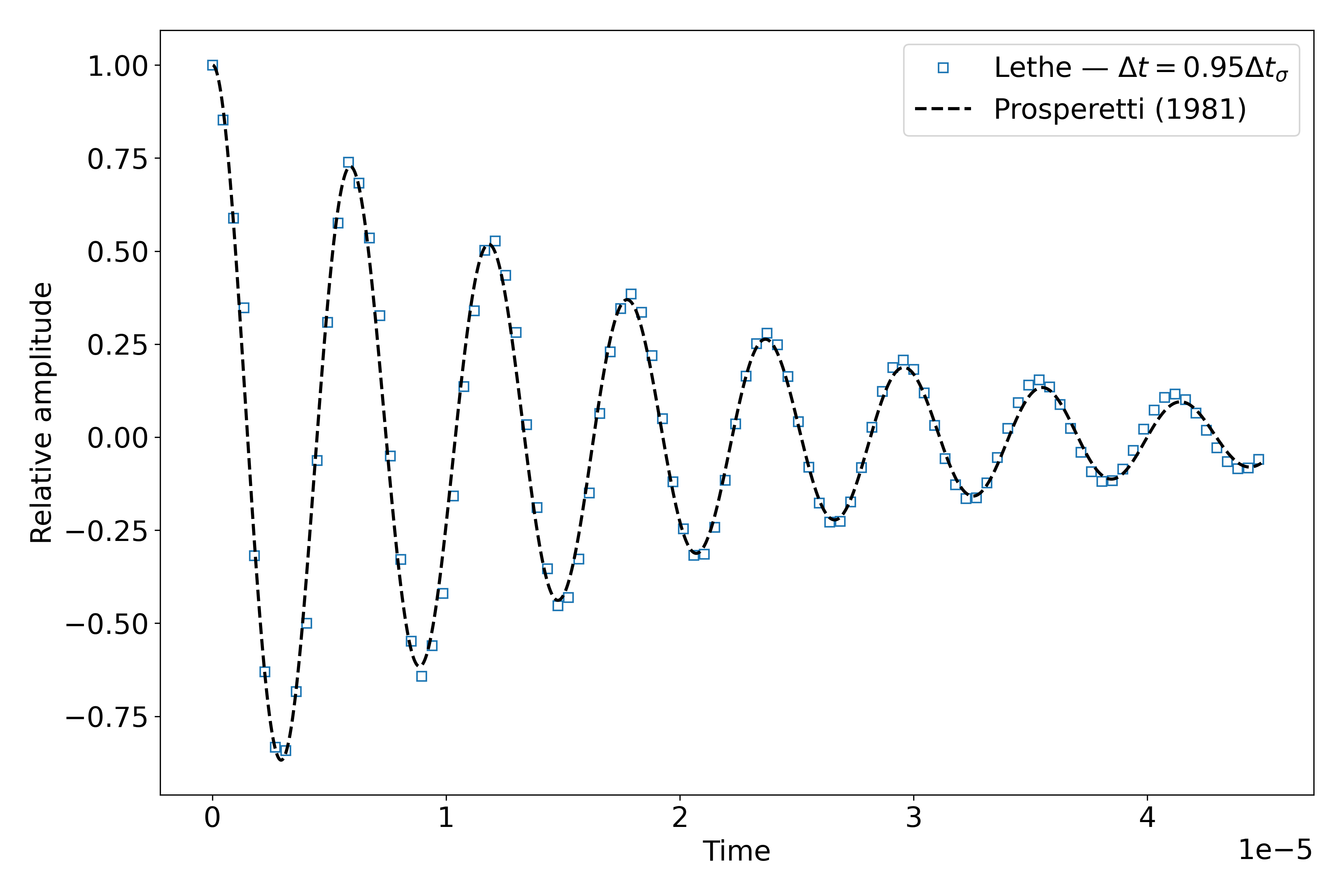
Wave relative amplitude evolution for \(\Delta t = 0.95\Delta t_\sigma\)

Results for \(\Delta t = \mathrm{TSM} \times \Delta t_\sigma\) with \(\mathrm{TSM} \in \{0.95,15,20\}\)

A comparison figure for multiple time-steps can be generated using the capillary-wave-combined.py Python script:

python3 capillary-wave-combined.py ./capillaryWaveData_rho_1_nu_5e-6_prosperetti.csv 0.95 15 20

with ./capillaryWaveData_rho_1_nu_5e-6_prosperetti.csv being the path to the analytical solution csv file and the following arguments are the \(\mathrm{TSM}\) you wish to add to your figure.

Warning

Before running capillary-wave-combined.py, data from individual cases must be extracted using capillary-wave-postprocess.py as shown in the subsection above.

Tip

If you want to prostprocess multiple cases consecutively and generate the comparison figure in one entry, a Bash script (capillary-wave-time-step-sensitivity-postprocess.sh) is provided. Make sure that the file has executable permissions before calling it using:

./capillary-wave-time-step-sensitivity-postprocess.sh ./capillaryWaveData_rho_1_nu_5e-6_prosperetti.csv "{0.95,15,20}" -sa

with ./capillaryWaveData_rho_1_nu_5e-6_prosperetti.csv being the path to the analytical solution csv file and "{0.95,15,20}" the sequence of \(\mathrm{TSM}\) of the different cases to postprocess. The last argument, -sa, stands for solve analytical, if this argument is added to the command, it will solve the analytical solution before postprocessing the results.

The following figure presents a comparison between the analytical results and the simulation results for \(\Delta t = \mathrm{TSM} \times \Delta t_\sigma\) with \(\mathrm{TSM} \in \{0.95,15,20\}\).

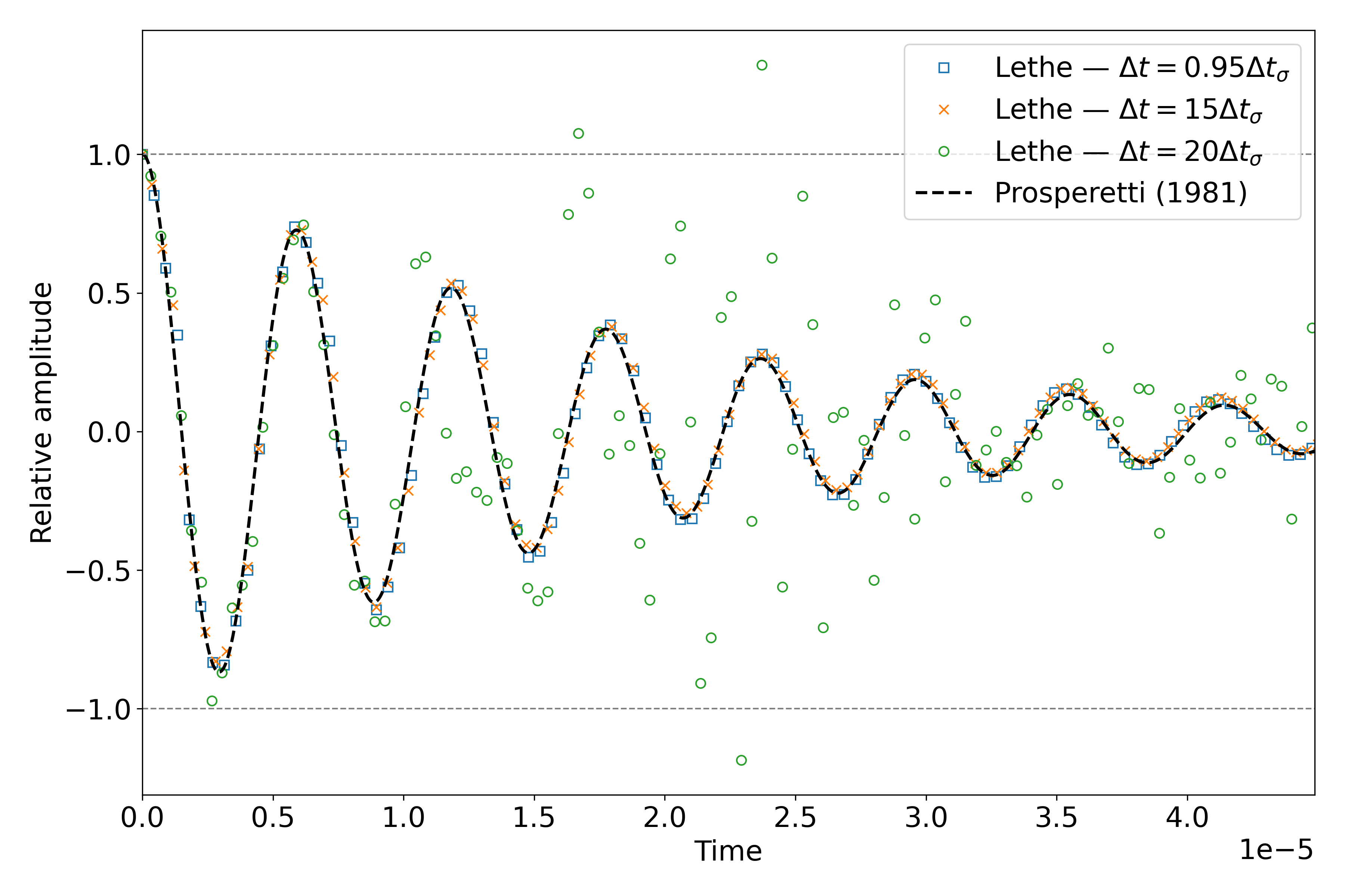
Comparison of wave relative amplitude evolutions for different time-steps for \(\mathrm{Oh=0.057}\) at the interface

A pretty good agreement is obtained for the \(2\) first simulations, demonstrating the accuracy and robustness of the VOF solver. The unexpected stability of the solution at \(\Delta t \approx 15\Delta t_\sigma\) is most probably the consequence of the implicit PSPG and SUPG stabilizations in the Navier-Stokes equations acting as artificial viscosity terms. These artificial viscosities locally increase the Ohnesorge number \(\left( \mathrm{Oh} = \frac{\mu_0+\mu_1}{\sqrt{2\hat{\rho}\sigma\Delta x}} \sim \frac{\text{viscous forces}}{\sqrt{\text{inertia} \times \text{surface tension}}}\right)\) near the interface which can be correlated to the stability of the simulation. As \(\mathrm{Oh}\) increases, it was found that the simulation results remain stable at higher multiples of the capillary time-step constraint [1, 2].

By increasing the mesh resolution by an additional refinement, the \(\mathrm{Oh}\) at the interface increases, therefore viscous effects increase and we get a more stable solution as seen below. However, we also see a slight negative phase shift.

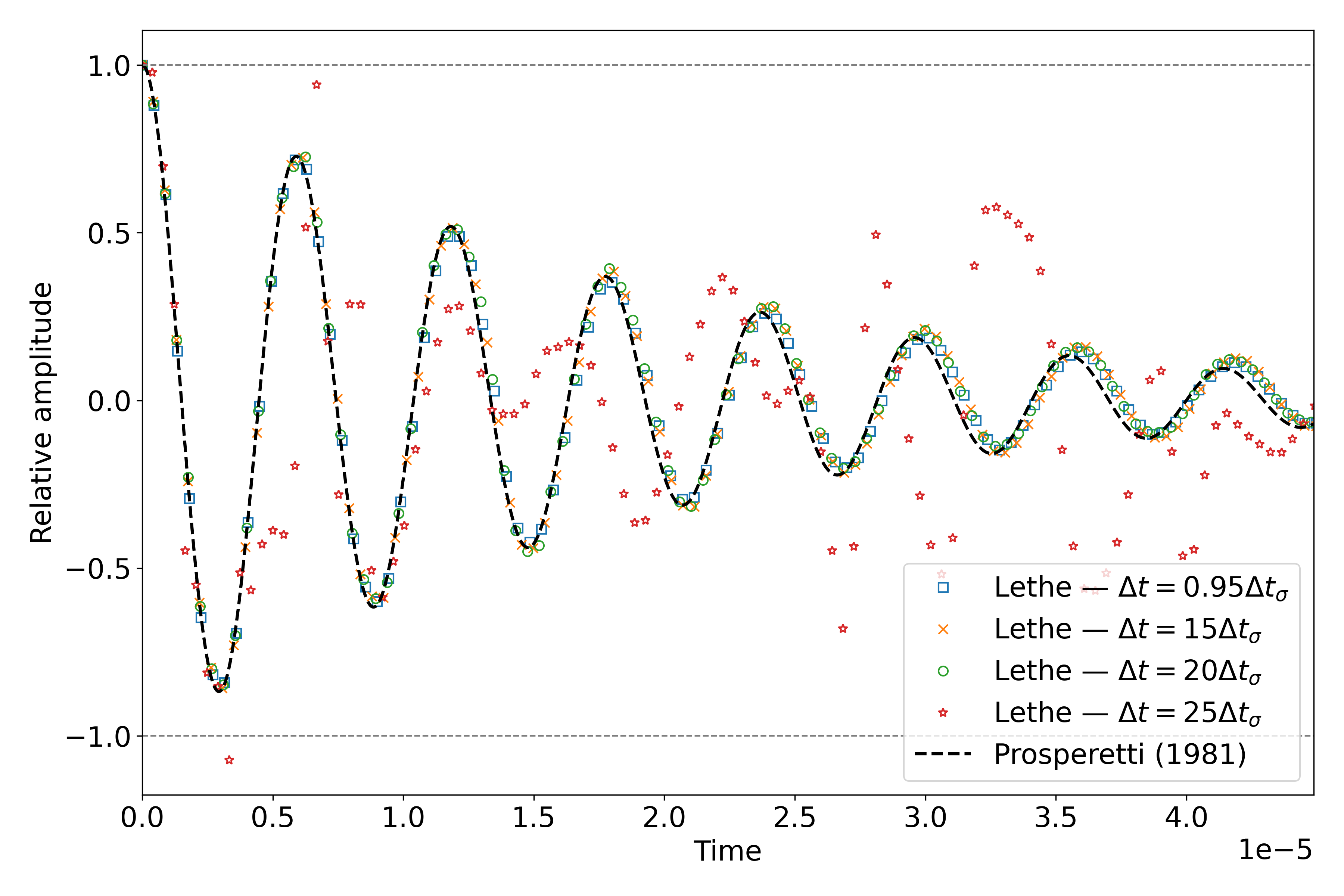
Comparison of wave relative amplitude evolutions for different time-steps for \(\mathrm{Oh=0.08}\) at the interface

Acknowledgment

We would like to thank Prof. Fabian Denner for sharing his time and knowledge throughout the process of developing this example.

References

[1]

F. Denner, F. Evrard, and B. van Wachem, “Breaching the capillary time-step constraint using a coupled VOF method with implicit surface tension,” J. Comput. Phys., vol. 459, p. 111128, Jun. 2022, doi: 10.1016/j.jcp.2022.111128.

[2]

F. Denner and B. G. M. van Wachem, “Numerical time-step restrictions as a result of capillary waves,” J. Comput. Phys., vol. 285, pp. 24–40, Mar. 2015, doi: 10.1016/j.jcp.2015.01.021.

[3]

A. Prosperetti, “Motion of two superposed viscous fluids,” Phys. Fluids, vol. 24, no. 7, pp. 1217–1223, Jul. 1981, doi: 10.1063/1.863522.