Heat Transfer in Aligned Particles#

This example introduces the use of multiphysic DEM with a simple example that consists of lined up particles that are heated by others or by a wall. It verifies the models of particle-particle and particle-wall heat transfer using two simple test cases.

Features#

Solvers: lethe-particles
Multiphysic DEM
Three-dimensional problem
Moving solid surfaces
Heating solid surface
Post-processing using Python, PyVista, lethe_pyvista_tools, and ParaView.

Files Used in This Example#

All files mentioned below are located in the example’s folder (examples/dem-mp/3d-heat-transfer-in-aligned-particles).

Parameter files: equilibrium.prm, wall-heating.prm
Geometry files solid surfaces: square-left.geo, square-right.geo
Input files: particles-equilibrium.input, particles-wall-heating.input
Post-processing Python scripts: equilibrium-postprocessing.py, wall-heating-postprocessing.py

Description of the Cases#

In the first stage of both simulations, 10 particles are put in contact. The solid surfaces on the left and right move towards the center to compress the particles, until they are all in contact on a line.

In the case of the equilibrium simulation, particles on the left side have a temperature of \(-30°C\) and particles on the right side have a temperature of \(30°C\). When all the particles are in contact on a line, the mean temperatures of the particles on the left and the particles on the right should vary towards the whole mean temperature, i.e. \(0°C\) here.

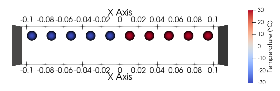
../../../_images/equilibrium-start.png — Temperatures at the start of the equilibrium simulation#

In the case of the wall-heating simulation, all particles start with a temperature of \(0°C\). The walls also have a temperature of \(0°C\). When all the particles are in contact on a line (\(t=8 s\)), the temperature of the right wall is set to \(50°C\). After some time, the temperature of the particles should be a linear function of their position.

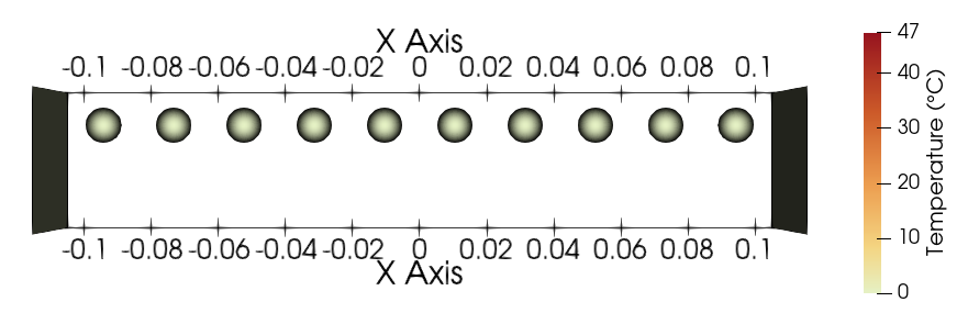
../../../_images/wall-heating-start.png — Temperatures at the start of the wall-heating simulation#

Parameter File#

Mesh#

The domain we simulate is a rectangular box with dimensions \(0.30\times0.05\times0.5\) meters and is made using the deal.ii grid generator.

subsection mesh
  set type               = dealii
  set grid type          = hyper_rectangle
  set grid arguments     = -0.15 , -0.025 , -0.025 : 0.15 , 0.025 , 0.025 : false
  set initial refinement = 1
end

Lagrangian Physical Properties#

The \(10\) particles are mono-dispersed, with a diameter of \(10\) mm.

Some parameters used in multiphysic DEM, like the thermal conductivity and specific heat, were chosen to ensure the simulations are fast enough, as simulations involving temperature can take up a lot of time to reach a steady state. Since these test cases are focused on temperature, and particles are set on a horizontal line, gravity is not taken into account.

subsection lagrangian physical properties
  set g                        = 0.0, 0.0, 0.0
  set number of particle types = 1
  subsection particle type 0
    set size distribution type            = uniform
    set diameter                          = 0.01
    set number of particles               = 10
    set density particles                 = 2500
    set young modulus particles           = 1e6
    set poisson ratio particles           = 0.3
    set restitution coefficient particles = 0.3
    set friction coefficient particles    = 0.3
    set rolling friction particles        = 0.3
    set thermal conductivity particles    = 3000
    set specific heat particles           = 300
    set microhardness particles           = 1.e9
    set surface slope particles           = 0.1
    set surface roughness particles       = 1.e-9
    set thermal accommodation particles   = 0.7
  end
  set young modulus wall           = 1e6
  set poisson ratio wall           = 0.3
  set restitution coefficient wall = 0.3
  set friction coefficient wall    = 0.3
  set rolling friction wall        = 0.3
  set thermal conductivity gas     = 0.2
  set specific heat gas            = 10000
  set dynamic viscosity gas        = 9.e-6
  set specific heats ratio gas     = 1.4
  set molecular mean free path gas = 68.e-9
  end

Model Parameters#

subsection model parameters
  subsection contact detection
    set contact detection method                = dynamic
    set dynamic contact search size coefficient = 0.9
    set neighborhood threshold                  = 1.3
  end
  set particle particle contact force method = hertz_mindlin_limit_overlap
  set rolling resistance torque method       = constant_resistance
  set particle wall contact force method     = nonlinear
  set integration method                     = velocity_verlet
  set solver type                            = dem_mp
end

Particle Insertion#

Since the simulations only involve \(10\) particles, they were inserted at precise locations using the file insertion method and input files particles-wall-heating.input for the wall-heating simulation and particles-equilibrium.input for the equilibrium simulation.

subsection insertion info
  set insertion method                               = file
  set insertion frequency                            = 10000
  set list of input files                            = particles-wall-heating.input
end

subsection insertion info
  set insertion method                               = file
  set insertion frequency                            = 10000
  set list of input files                            = particles-equilibrium.input
end

Solid Objects#

For the equilibrium simulation, walls are considered adiabatic and move towards the center until they reach their set location.

subsection solid objects
  subsection solid surfaces
    set number of solids = 2
    subsection solid object 0
      subsection mesh
        set type               = gmsh
        set file name          = square-left.msh
        set simplex            = true
        set initial refinement = 0
      end
      subsection translational velocity
        set Function expression = if(x<-0.049,0.01,0) ; 0 ; 0
      end
      subsection angular velocity
        set Function expression = 0 ; 0 ; 0
      end
      set center of rotation    = -0.11 , 0 , 0
      set thermal boundary type = adiabatic
    end
    subsection solid object 1
      subsection mesh
        set type               = gmsh
        set file name          = square-right.msh
        set simplex            = true
        set initial refinement = 0
      end
      subsection translational velocity
        set Function expression = if(x>0.049,-0.01,0) ; 0 ; 0
      end
      subsection angular velocity
        set Function expression = 0 ; 0 ; 0
      end
      set center of rotation    = 0.11 , 0 , 0
      set thermal boundary type = adiabatic
    end
  end
end

For the wall-heating simulation, walls have a uniform temperature (isothermal) and move towards the center until they reach their set location.

subsection solid objects
  subsection solid surfaces
    set number of solids = 2
    subsection solid object 0
      subsection mesh
        set type               = gmsh
        set file name          = square-left.msh
        set simplex            = true
        set initial refinement = 0
      end
      subsection translational velocity
        set Function expression = if(x<-0.045,0.01,0) ; 0 ; 0
      end
      subsection angular velocity
        set Function expression = 0 ; 0 ; 0
      end
      set center of rotation    = -0.11 , 0 , 0
      set thermal boundary type = isothermal
      subsection temperature
        set Function expression = 0
      end
    end
    subsection solid object 1
      subsection mesh
        set type               = gmsh
        set file name          = square-right.msh
        set simplex            = true
        set initial refinement = 0
      end
      subsection translational velocity
        set Function expression = if(x>0.045,-0.01,0) ; 0 ; 0
      end
      subsection angular velocity
        set Function expression = 0 ; 0 ; 0
      end
      set center of rotation    = 0.11 , 0 , 0
      set thermal boundary type = isothermal
      subsection temperature
        set Function expression = if(t>8,50,0)
      end
    end
  end
end

Simulation Control#

The simulations run for 20 and 15 seconds of real time, respectively. We output the simulation results every 10000 iterations.

subsection simulation control
  set time step         = 5e-5
  set time end          = 20
  set log frequency     = 10000
  set output frequency  = 10000
  set output path       = ./output_equilibrium/
  set output boundaries = true
end

subsection simulation control
  set time step         = 5e-5
  set time end          = 15
  set log frequency     = 10000
  set output frequency  = 10000
  set output path       = ./output_wall_heating/
  set output boundaries = true
end

Running the Simulation#

The simulations can be launched with

 lethe-particles equilibrium.prm

 lethe-particles wall-heating.prm

Note

Parallel calculations are not necessary here as there are only \(10\) particles.

Post-processing#

A Python post-processing code is provided for each case: equilibrium-postprocessing.py and wall-heating-postprocessing.py.

The first post-processing script is used to check that the two mean temperatures (of particles with \(x<0\) and \(x>0\)) do get close to the global mean temperature at the end of the equilibrium simulation.

The second script is used to confirm that the temperature of the particles matches the analytical solution \(T(x) = Ax+B\), where \(A\) and \(B\) are found using the temperature and position that are set for the left and right walls.

It is possible to run the post-processing codes with the following commands. The argument is the folder which contains the .prm file.

  python3 equilibrium-postprocessing.py  --folder ./

  python3 wall-heating-postprocessing.py  --folder ./

Important

You need to ensure that lethe_pyvista_tools is working on your machine. Click here for details.

Results#

Results for the Equilibrium Simulation#

The simulation can be visualised using Paraview as seen below.

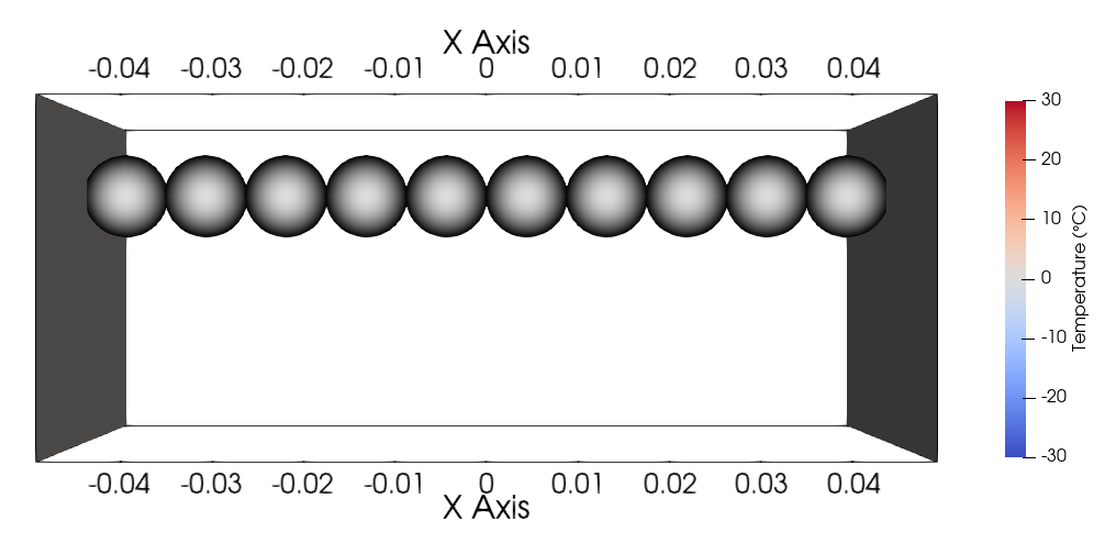
../../../_images/equilibrium.png — Temperatures at the end of the simulation#

The following figure shows that the two mean temperatures do converge towards \(0°C\), as expected.

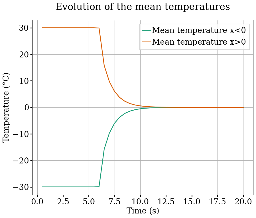
It was noticed while choosing the parameters for the simulation that the more the walls compress the particles, the faster the mean temperatures reach \(0°C\). This highlights the importance of the overlap in the particle-particle and particle-wall heat transfer models.

Results for the Wall-heating Simulation#

The simulation can be visualised using Paraview as seen below.

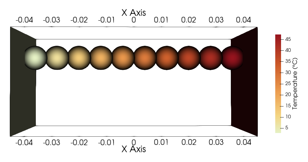
../../../_images/wall-heating.png — Temperatures at the end of the simulation#

The following figure compares the temperatures of the particles at the end of the simulation with the analytical solution \(T(x) = Ax+B\).

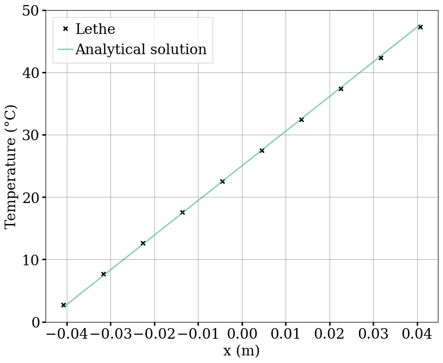
The results show very good agreement with the analytical solution.