Cooling Fin

This example simulates the heat transfer in a cooling fin, which is a classical problem in heat transfer

Features

• Solver: lethe-fluid

• Heat transfer

• Usage of a python script for post-processing data

Files Used in This Example

Both files mentioned below are located in the example’s folder (examples/multiphysics/cooling-fin).

• Parameter file: fin.prm

• Postprocessing python script: compare_solution.py

Description of the Case

A cylindrical fin of length \(L=0.2\) and radius \(R=0.01\) is fixed to a wall at a constant temperature \(T_b=100\). The radial surface of the fin is subject to natural convection following Newton’s law of cooling with \(h=10\) and \(T_{\infty}=20\). The material from which the fin is made has a thermal conductivity \(k=100\mathrm{W/m/K}\). The geometry of this example is illustrated below.

In the case where the Biot number \(\mathrm{Bi}=\frac{hR}{k}<1\), the temperature distribution in the fin can be assumed to vary only along the \(x\) direction and is approximated very adequately by the following equation [1]:

\[T(x) = T_\infty + (T_b - T_\infty) \frac{\cosh(\beta(L-x))}{\cosh(\beta L)}\]

where \(\beta=\sqrt{\frac{hP}{kA}}\) is the fin parameter, \(P\) is the perimeter of the fin, and \(A\) is the cross-sectional area of the fin.

Parameter File

Simulation Control

The simulation is done in steady state without mesh adaptation.

subsection simulation control
  set method           = steady
  set output name      = out
  set output path      = ./output/
end

Multiphysics

The multiphysics subsection is used to to disable fluid dynamics and enable the heat transfer physics.

subsection multiphysics
  set fluid dynamics = false
  set heat transfer  = true
end

Boundary Conditions

Boundary conditions must be set for both fluid dynamics and heat transfer, even though the former is not used.

Boundary Conditions - Fluid Dynamics

For the fluid dynamics, we set the boundary conditions to no-slip on all the boundaries.

subsection boundary conditions
  set number = 3
  subsection bc 0
    set id    = 0
    set type  = noslip
  end
  subsection bc 1
    set id    = 1
    set type  = noslip
  end
  subsection bc 2
    set id    = 2
    set type  = noslip
  end
end

Boundary Conditions - Heat Transfer

For the heat transfer, we set the boundary conditions as follows:

subsection boundary conditions heat transfer
  set number = 3
  subsection bc 0
    set id    = 0
    set type = convection-radiation-flux
    subsection h
      set Function expression = 10
    end
    subsection Tinf
      set Function expression = 20
    end
    subsection emissivity
      set Function expression = 0
    end
    subsection heat_flux
      set Function expression = 0
    end
  end
  subsection bc 1
    set id    = 1
    set type  = temperature
    subsection value
      set Function expression = 100
    end
  end
  subsection bc 2
    set id    = 2
    set type = convection-radiation-flux
    subsection h
      set Function expression = 0
    end
    subsection Tinf
      set Function expression = 20
    end
    subsection emissivity
      set Function expression = 0
    end
    subsection heat_flux
      set Function expression = 0
    end
  end
end

Physical Properties

In the physical properties subsection, we define the properties of the fin. The thermal conductivity is set to \(k=100\). Even though the fin is technically a solid, by default Lethe calls fluid the material which is used in the simulation domain when there is only one material.

subsection physical properties
  set number of fluids = 1
  subsection fluid 0
    set thermal conductivity       = 100
  end
end

Mesh

In the mesh subsection, we define a cylinder with the appropriate dimensions. We use the subdivided_cylinder grid generator to manually control the number of division on the axial direction of the cylinder. The mesh is initially refined \(3\) times to ensure that it is sufficiently fine.

subsection mesh
  set type               = dealii
  set grid type          = subdivided_cylinder
  set grid arguments     = 10 : 0.01 : 0.1
  set initial refinement = 3
end

FEM

We use the FEM subsection to define the order of the finite element method used in the simulation. We set the order to 2 for the temperature field.

subsection FEM
  set temperature order = 2
end

Postprocessing

We calculate the heat fluxes on the boundaries of the fin.

subsection post-processing
  set verbosity                        = verbose
  set calculate heat flux              = true
end

Running the Simulation

We can call lethe-fluid by invoking the following command:

lethe-fluid fin.prm

Note

This simulation should take less than a minute if Lethe is compiled in release mode

Results

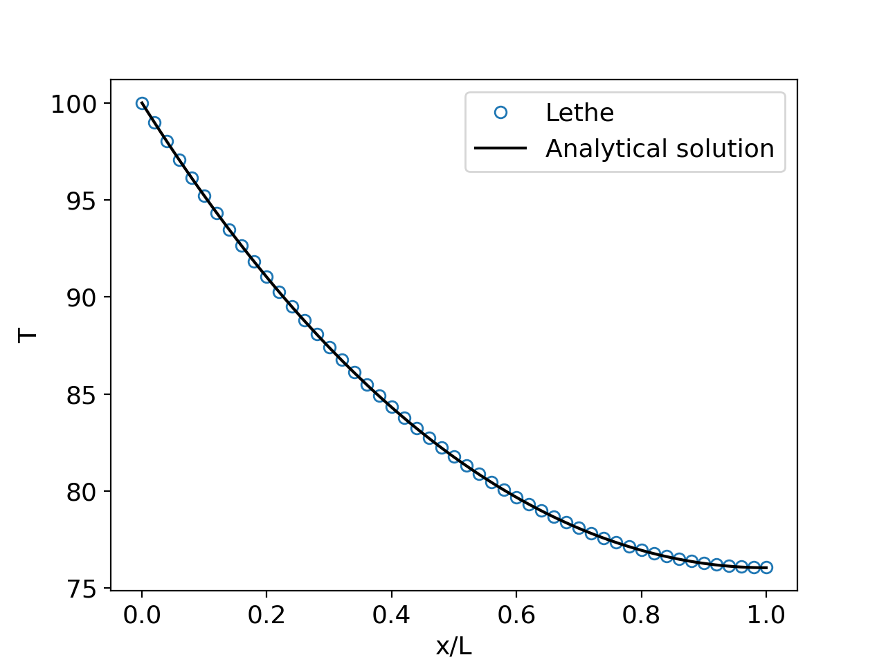
A postprocessing script is provided with the example. It extracts the axial temperature profile in the fin and compares it with the analytical solution. The script can be run by invoking the following command and specifying the vtu output file:

python3 compare_solution.py --vtu output/out.00001.00000.vtu

The following figure shows the temperature distribution in the fin. The analytical solution is also plotted for comparison. The agreement between the simulation and analytical results is excellent.

The postprocessing script also calculates the heat fluxes on the boundaries of the fin. The following table shows the heat fluxes calculated by the simulation and the analytical solution.

Boundary	Simulation (W)	Analytical (W)
Radial surface of the fin	8.019	8.020
Base of the fin	8.019	8.020

We see that even with a relatively coarse mesh, the heat fluxes calculated by the simulation are very close to the analytical solution.

Possibilities for Extension

• The heat flux is sensitive to the finite element order used for the temperature field. Try the simulations again with first-order Q1 elements and compare the results.

References

[1]

R. B. Bird, W. E. Stewart, and E. N. Lightfoot, Transport Phenomena, vol. 1. John Wiley & Sons, 2006.