Rayleigh-Bénard Convection

This example simulates a two-dimensional Rayleigh–Bénard convection [1] [2] [3] at Rayleigh numbers of \(10^4\) and \(10^6\) .

Features

• Solver: lethe-fluid

• Buoyant force (natural convection)

• Unsteady problem handled by an adaptive BDF1 time-stepping scheme

Files Used in This Example

Both files mentioned below are located in the example’s folder (examples/multiphysics/rayleigh-benard-convection).

• Parameter file for \(Ra=10^4\): rayleigh-benard-convection-Ra10k.prm

• Parameter file for \(Ra=10^6\): rayleigh-benard-convection-Ra1M.prm

Description of the Case

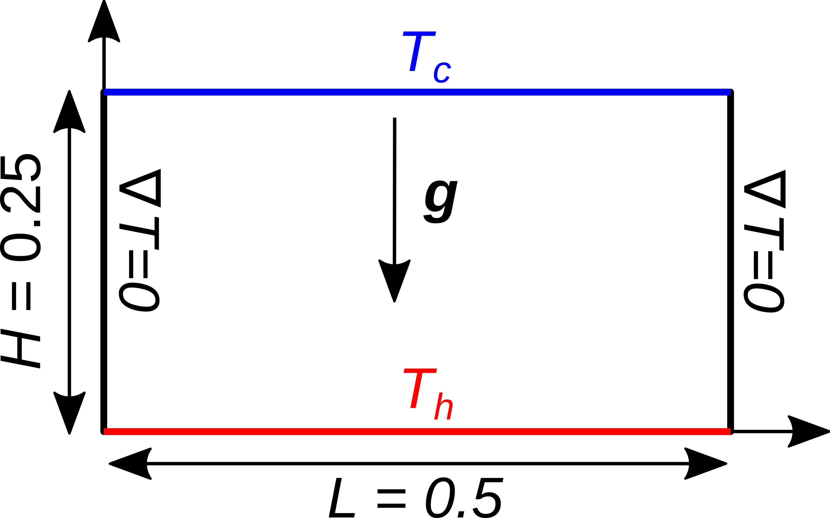
In this example, we evaluate the performance of the lethe-fluid solver in the simulation of the stability of natural convection within a two-dimensional square domain. Our results are tested against the benchmark presented by Ouertatani et al. [1] . The following schematic describes the geometry and dimensions of the simulation:

The incompressible Navier-Stokes equations with a Boussinesq approximation for the buoyant force are:

\[\begin{split}\nabla \cdot {\bf{u}} &= 0 \\ \rho \frac{\partial {\bf{u}}}{\partial t} + \rho ({\bf{u}} \cdot \nabla) {\bf{u}} &= -\nabla p + \nabla \cdot {\bf{\tau}} - \rho \beta {\bf{g}} (T - T_0)\end{split}\]

where \(\beta\) and \(T_0\) denote thermal expansion coefficient and a reference temperature, respectively.

A two-dimensional block of fluid is heated from its bottom wall at \(t = 0\) s. The temperature of the bottom wall is equal to \(T_\text{h}=10\), the temperature of the top wall is equal to \(T_\text{c}=0\), and the left and right walls are insulated. By heating the fluid from the bottom wall, the buoyant force (natural convection) creates vortices inside the fluid. The shape and count of these vortices depend on the Rayleigh number and the Prandtl dimensionless numbers [1] [2] :

\[\begin{split}Ra &= \frac{\rho^2 \beta g (T_\text{h} - T_\text{c}) H^3 c_\text{p}}{k \mu} \\ Pr &= \frac{\mu c_\text{p}}{k}\end{split}\]

where \(\rho\) is the fluid density, \(g\) is the magnitude of gravitational acceleration, \(H\) denotes the characteristic length, \(k\) is the thermal conduction coefficient, \(\mu\) is the dynamic viscosity, and \(c_\text{p}\) is the specific heat capacity.

In this example, we simulate the Rayleigh-Bénard convection problem at two Rayleigh numbers ( \(Ra=10^4\) and \(Ra=10^6\) ) with a Prandtl number of \(Pr=0.71\) which correspond to air. According to the literature [1] , we should see one big convective cell at steady-state for both \(Ra=10^4\) and \(Ra=10^6\), but for the latter, there should also be two small vortices in opposite corners rotating in the reverse direction of the big vortex. For simplicity, the gravity magnitude is set to 10 pointing in the opposite direction of the y-axis for both simulations. Additionally, because the two dimensionless numbers above are the only thing that characterize the flow we may choose the remaining parameters as we want. Here we chose to fix \(\rho = 1\), \(H = 1\), \(c_\text{p} = 100\) and \(\mu = 0.071\). Thus, the Rayleigh number is controlled only by the thermal expansion coefficient (\(\beta = 0.71\) or \(\beta = 71\)).

Note

All four boundary conditions for the velocity are noslip. The sides wall are set to convection-radiation-flux with a heat transfer coefficient of 0 to have isolated walls. The top and bottom walls are set to a temperature to force a value of 0 and 10, respectively.

Parameter File

For simplicity, we present only the parameter file for \(Ra=10^4\).

Note

Note that the resolution (256x256) is set to match the one of the article results [1] . If desired, you can choose to reduced to 7 or 6 the initial refinement level in the parameter files to reduce the simulation time without loosing too much accuracy.

Simulation Control

The time integration is handled by a 1st order backward differentiation scheme (bdf1). A simulation time of \(24\) s has been selected to ensure that the system reaches a quasi-steady state. The initial time-step is set to \(0.001\) s, but this will be adapted during the simulation.

Note

This example uses an adaptive time-stepping method, where the time-step is modified during the simulation to keep the maximum value of the CFL condition below a given threshold (0.9 here). Using output control = time, and output time frequency = 0.5 the simulation results are written every 0.5 seconds regardless of the time-steps.

subsection simulation control
  set method                       = bdf1
  set time end                     = 24
  set time step                    = 0.01
  set adapt                        = true
  set max cfl                      = 0.9
  set stop tolerance               = 1e-5
  set adaptative time step scaling = 1.3
  set number mesh adapt            = 0
  set output name                  = rayleigh-benard_convection
  set output control               = time
  set output time frequency        = 0.5
  set output path                  = ./output/
end

Multiphysics

The multiphysics subsection enables to turn on true and off false the physics of interest. Here heat transfer, buoyancy force, and fluid dynamics are chosen.

subsection multiphysics
  set buoyancy force = true
  set heat transfer  = true
  set fluid dynamics = true
end

Source Term

The source term subsection defines gravitational acceleration.

subsection source term
  subsection fluid dynamics
    set Function expression = 0 ; -10 ; 0
  end
end

Physical Properties

The physical properties subsection defines the physical properties of the fluid.

subsection physical properties
  set number of fluids = 1
  subsection fluid 0
    set density              = 1
    set kinematic viscosity  = 0.071
    set thermal expansion    = 0.71
    set thermal conductivity = 10
    set specific heat        = 100
  end
end

Running the Simulation

Call the lethe-fluid by invoking:

mpirun -np 8 lethe-fluid rayleigh-benard-convection-Ra10k.prm

or

mpirun -np 8 lethe-fluid rayleigh-benard-convection-Ra1M.prm

to run the simulations using eight CPU cores for the \(Ra=10^4\) and \(Ra=10^6\) cases respectively. Feel free to use more CPU if available.

Warning

Make sure to compile lethe in Release mode and run in parallel using mpirun. The first simulation takes \(\approx\) 20 minutes on 8 processes and the second at \(Ra=10^6\) can take a few hours because of the much smaller time-step required to respect the CFL condition.

Results

The following animation shows the evolution of the temperature field with the flow direction for the simulation at \(Ra=10^6\):

Below, we also present the velocity profiles at steady-state of our simulation compared to the ones presented by Ouertatani et al. [1] as a verfification of the Lethe software.

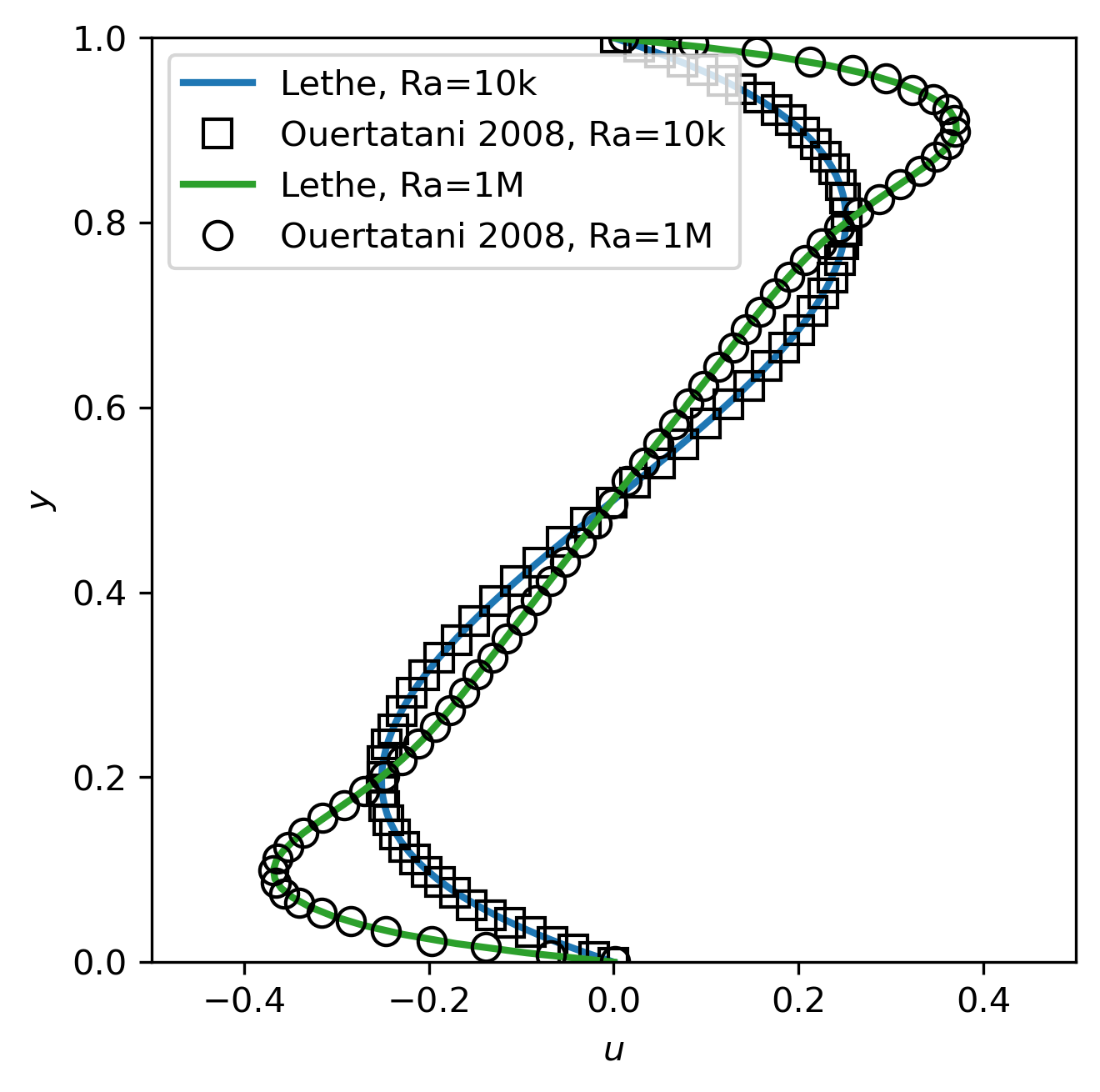
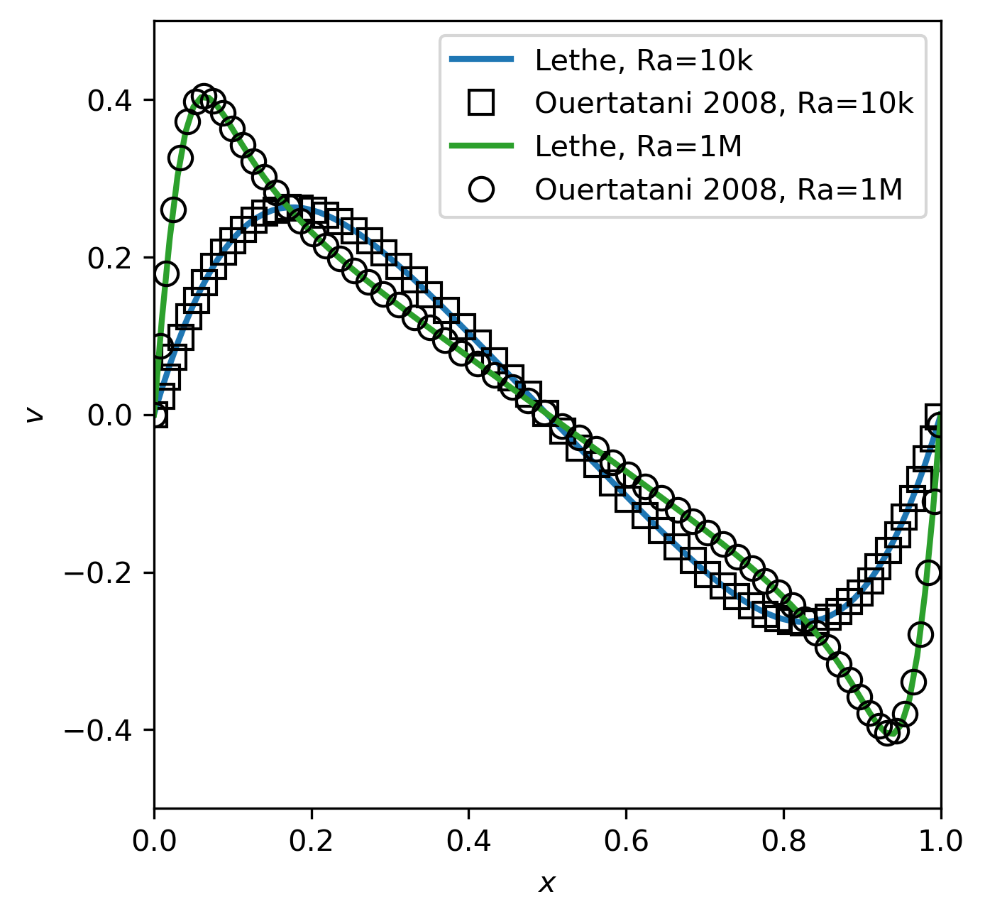
The results can be postprocessed using the provided Python script (rayleigh-benard-convection.py). Here is an example of how to call the script:

python3 rayleigh-benard-convection.py -f ./output_10k -f ./output_1M -Ra 10k -Ra 1M

This script extracts the velocity in the \(x\) and \(y\) directions at the mid-width (\(x=0.5\)) and mid-height (\(y=0.5\)) respectively and create the above plots.

Warning

The orientation of the vortex rotation obtained with the simulation may differ from the one above due to machine precision that generates the initial instability.

Important

You need to ensure that the lethe_pyvista_tools is working on your machine. Click here for details.

References

[1] (1,2,3,4,5,6)

N. Ouertatani, N. Ben Cheikh, B. Ben Beya, T. Lili, “Numerical simulation of two-dimensional Rayleigh-Bénard convection in an enclosure,” Comptes Rendus – Mec. 2008;336(5):464–70. 10.1016/j.crme.2008.02.004.

[2] (1,2)

D. Venturi, X. Wan, and G. E. Karniadakis, “Stochastic bifurcation analysis of Rayleigh–Bénard convection,” J. Fluid Mech., vol. 650, pp. 391–413, May 2010, doi: 10.1017/S0022112009993685.

[3]

“Rayleigh-Bénard Convection” Max Planck Institute, Accessed: 17 Jul. 2024, Available: https://archive.ph/XrJXx.