Rotating Drum#
This example simulates a rotating drum. We setup this simulation according to the experiments of Alizadeh et al. [1] It is recommended to visit DEM parameters for more detailed information on the concepts and physical meanings of the parameters in Lethe-DEM.
Features#
Solvers:
lethe-particlesRotational boundary
Load-balancing
Files Used in This Example#
Both files mentioned below are located in the example’s folder (examples/dem/3d-rotating-drum).
Parameter file to load particles:
load-rotating-drum.prmParameter file for the simulation:
rotating-drum.prm
Description of the Case#
226080 particles are first inserted into a cylindrical domain and then start rolling on the cylinder wall because of the rotation of the cylinder. This rotation is applied using a rotational boundary condition. Because of the large number of particles, this simulation should be launched in parallel mode with load-balancing. The concepts and different types of boundary condition and load-balancing are explained in this example.
Parameter File#
Mesh#
In this example, we choose a cylinder grid type to create a cylinder. Grid arguments are the radius and half-length, respectively. Therefore, the specified grid arguments create a cylinder with a diameter of 0.24 m and a length of 0.36 m. The grid is refined 4 times to reach the desired cell size to particle diameter ratio (see packing in ball example for more details). The expand particle-wall contact search is used in concave geometries to enable extended particle-wall contact search with boundary faces of neighbor cells for particles located in each boundary cell.
subsection mesh
  set type                                = dealii
  set grid type                           = subdivided_cylinder
  set grid arguments                      = 4: 0.12:0.18
  set initial refinement                  = 4
  set expand particle-wall contact search = true
end
Insertion Info#
An insertion box is defined inside the cylindrical domain. 38000 particles are inserted non-uniformly at each insertion step.
subsection insertion info
  set insertion method                               = volume
  set inserted number of particles at each time step = 38000
  set insertion frequency                            = 25000
  set insertion box points coordinates               = -0.175, -0.07, 0 : 0.175, 0.07, 0.09
  set insertion distance threshold                   = 1.575
  set insertion maximum offset                       = 0.025
  set insertion prn seed                             = 19
end
Lagrangian Physical Properties#
The particles are monodispersed. Their diameter and density are 0.003 m and 2500 kg/m3 respectively.
subsection lagrangian physical properties
  set g                        = 0.0, 0.0, -9.81
  set number of particle types = 1
  subsection particle type 0
    set size distribution type            = uniform
    set diameter                          = 0.003
    set number of particles               = 226080
    set density particles                 = 2500
    set young modulus particles           = 1e7
    set poisson ratio particles           = 0.20
    set restitution coefficient particles = 0.97
    set friction coefficient particles    = 0.85
  end
  set young modulus wall           = 1e7
  set poisson ratio wall           = 0.20
  set restitution coefficient wall = 0.85
  set friction coefficient wall    = 0.85
end
Model Parameters#
Load-balancing updates the distribution of the subdomains between the processes in parallel simulation to achieve better computational performance (less simulation time). Three load-balancing methods are available in Lethe-DEM: once, frequent, or dynamic. Read this article for more information about different load-balancing methods and their performances in various types of DEM simulations.
In the rotating drum simulation, we use a frequent load-balancing method and repartition the particles every \(20 000\) iterations.
subsection model parameters
  subsection contact detection
    set contact detection method                = dynamic
    set dynamic contact search size coefficient = 0.8
    set neighborhood threshold                  = 1.3
  end
  subsection load balancing
    set load balance method = frequent
    set frequency           = 20000
  end
  set particle particle contact force method    = hertz_mindlin_limit_overlap
  set particle wall contact force method        = nonlinear
  set rolling resistance torque method          = none
  set integration method                        = velocity_verlet
end
DEM Boundary Conditions#
In this subsection, the boundary conditions of the DEM simulation are defined. First of all, the number of boundary conditions is specified. Then for each boundary condition, its information is defined. Using rotational boundary condition exerts imaginary rotational velocity to that boundary. In other words, the boundary does not move, but the particles that have collisions with these walls feel a rotational or translational velocity from the wall. This feature is used in the rotating drum example. The boundary id of the cylinder side wall, defined with deal.ii grid generator is 4. We set the rotational speed equal to 11.6 rad/s, and the cylinder should rotate on its axis (x direction).
subsection DEM boundary conditions
  set number of boundary conditions = 3
  subsection boundary condition 0
    set boundary id       = 0
    set type              = rotational
    set rotational speed  = 1.214749159
    set rotational vector = 1, 0, 0
  end
  subsection boundary condition 1
    set boundary id       = 1
    set type              = rotational
    set rotational speed  = 1.214749159
    set rotational vector = 1, 0, 0
  end
  subsection boundary condition 2
    set boundary id       = 2
    set type              = rotational
    set rotational speed  = 1.214749159
    set rotational vector = 1, 0, 0
  end
end
Simulation Control#
The parameter file for the loading and for the simulation have different simulation control. We load for two seconds, then simulate for 10 secondes (reaching a final time of 12 seconds).
For the loading the simulation control is:
subsection simulation control
  set time step         = 1e-5
  set time end          = 2
  set log frequency     = 1000
  set output frequency  = 1000
  set output boundaries = true
  set output path       = ./output/
end
For the simulation it is:
subsection simulation control
  set time step        = 1e-5
  set time end         = 10
  set log frequency    = 1000
  set output frequency = 1000
  set output boundaries = false
  set output path       = ./output/
end
Running the Simulation#
This simulation can be launched in two steps. First the particles need to be loaded (here we use 8 cores):
Then we run the simulation with the rotating walls:
Warning
In this example, particles insertion requires approximately 50 minutes, while simulating their motion requires additional 8 hours on 8 cores. The high computational cost is due to the large number of particles and the long duration of the simulation.
Results#
Animation of the rotating drum simulation:
We can compare the results of the simulation with the experimental results of Alizadeh et al. [1].
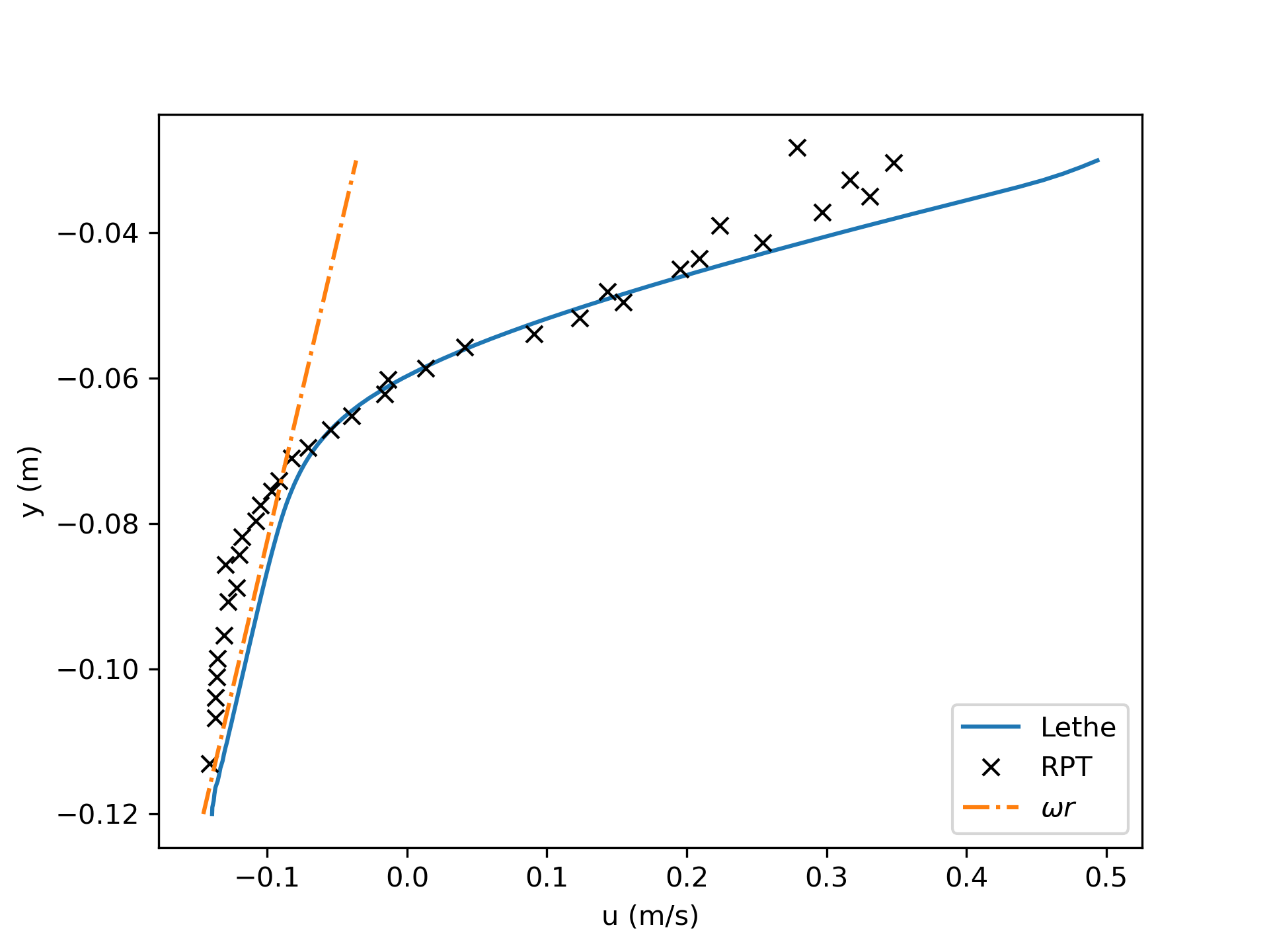
The following graph compares the velocity of the particles aligned with the slope of the heap as a function of the depth with the experimental results. We note that there is a good agreement between the simulation and the experimental results.
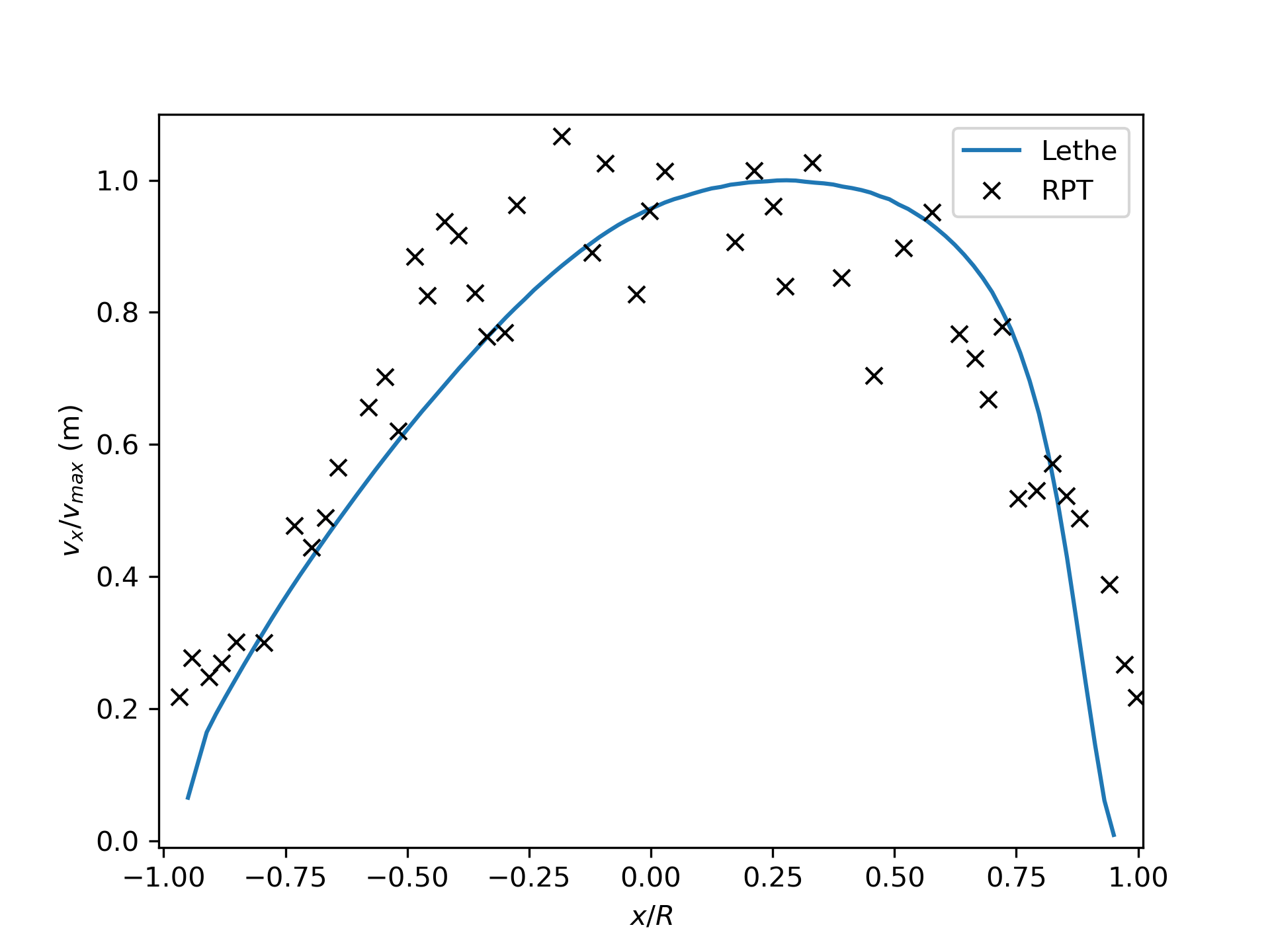
The following graph compares the velocity of the particles aligned with the slope of the heap on the free surface of the heap. Again, we note a very good agreement with the experimental results.