Bouncing Particle#
This example of Lethe simulates the bounces of a single particle using the linear spring-dashpot collision model in 3D. This simulation is being setup according to MFIX DEM02 verification test [1]. It is recommended to visit DEM parameters for more detailed information on the concepts and physical meanings of the parameters in Lethe.
Features#
Solvers:
lethe-particlesPostprocessing using Python, PyVista, lethe_pyvista_tools, and ParaView.
Files Used in This Example#
All files mentioned below are located in the example’s folder (examples/dem/3d-bouncing-particle).
Case generation Python script:
bouncing_particle_case_generator.pyParameter file for case generation:
bouncing_particle_original.tplPostprocessing Python script:
bouncing_particle_postprocessing.py
Description of the Case#
This simulation consists of a single particle bouncing on a flat plane. The particle is inserted at rest at a specific position and accelerates due to the action of gravity. Upon reaching the outer limit of the domain, the particle-wall contact stops the particles from leaving the triangulation. Depending on the values of spring constant and restitution coefficient used, the particle loses kinetic energy, thus the height of the next bounce decreases until the particle comes to a complete stop.
Parameter File#
Mesh#
The grid type in this example is a hyper_cube. Its dimensions are 2.0 m in every direction (from 0.0 m to 2.0 m), and since only one particle is used, the refinement is set to zero.
subsection mesh
  set type               = dealii
  set grid type          = hyper_cube
  set grid arguments     = 0.0 : 2.0 : false
  set initial refinement = 0
end
Insertion Info#
Since the insertion of the particle must be done at a specific location, the list insertion method is used. The insertion frequency can be set to any value, since we’re only using one particle. The insertion location is centered in the X-Y plane and at a height of 0.5 m in the Z direction.
subsection insertion info
  set insertion method     = list
  set insertion frequency  = 10000
  set list x               = 1.0
  set list y               = 1.0
  set list z               = 0.5
end
Lagrangian Physical Properties#
Different spring constant and restitution coefficient are used in this example. The spring constant is not defined explicitly in the parameter file, consequently the physical properties must be chosen to obtain a desired spring constant. The interested reader can consult DEM theory for more information about the definition of the sprint constant.
The poisson ratio of both the wall and the particle are being set to 0.3 arbitrarily. The Young’s modulus of the wall is also being set arbitrarily to the value of 1e3 GPa.
The following properties are defined in the bouncing_particle_original.tpl according to MFIX DEM02 verification test.
subsection lagrangian physical properties
  set g                        = 0.0, 0.0, -9.81
  set number of particle types = 1
  subsection particle type 0
    set size distribution type            = uniform
    set diameter                          = 0.2
    set number of particles               = 1
    set density particles                 = 2600
    set young modulus particles           = {{YP}}
    set poisson ratio particles           = 0.3
    set restitution coefficient particles = {{er}}
    set friction coefficient particles    = 0.0
  end
  set young modulus wall           = 1000000000000
  set poisson ratio wall           = 0.30
  set restitution coefficient wall = {{er}}
  set friction coefficient wall    = 0.
end
As you can see, the young modulus particles and the restitution coefficient of both the wall and particle are not yet defined in the bouncing_particle_original.tpl file. A Python code called bouncing_particle_case_generator.py is provided with this example which generates 6 parameter files each using different restitution coefficient values (from 0.5 to 1.0) for one specific normal spring constant. The young modulus particles parameter will be determined using a bisection algorithm to satisfy the desired normal spring constant. Assuming you have Python3 installed on your machine, this code can be launched using this next line:
Where 5000000 represent the normal spring constant that is desired for the simulations. This code will generate 6 files named bouncing_particle_XX.prm, where XX represent the value of the restitution coefficient used in it. (10 means restitution of 1.0)
Running the Simulation#
Once all 6 parameter file are created, the simulation can be launched one after the other using the following line (parallel mode is not recommend since there is only one particle):
All 6 simulations takes less than 2 minutes to run. Folders named according to the restitution coefficient of every simulation used will be generated (/out_xx).
Postprocessing#
A Python post-processing code called bouncing_particle_post_processing.py is provided with this example. It compares the height reached by the particle after each bounce with the analytical solution of a hard sphere bouncing on a flat plane. This analytical solution considers instantaneous collision between the particle and the wall, thus the maximum height of each bounce can be express by the following expression:
with \(k\) representing the \(k^{th}\) bounce, \(h_0\) the starting height and \(r_p\) the radius of the particle.
Once all 6 simulations have been run, use the following line in your terminal to run the post-processing code :
Important
You need to ensure that lethe_pyvista_tools is working on your machine. Click here for details.
A figure will be generated which compares the analytical solution with the simulation results.
Results and Discussion#
Animation of a bouncing particle with different restitution coefficient (\(K_n\) = 5E6 N/m):
The particle with a restitution coefficient (\(e\)) of 1.0 always rebounds at the same height. Other particles show a reduction in rebound height which follows the analytical solution expressed earlier.
Using the post-processing code, it is possible to compare the effect of the normal spring constant of the conservation of the kinetic energy during the collision.

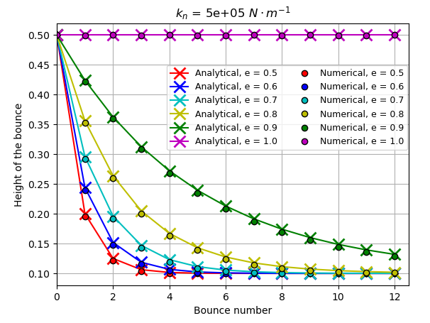
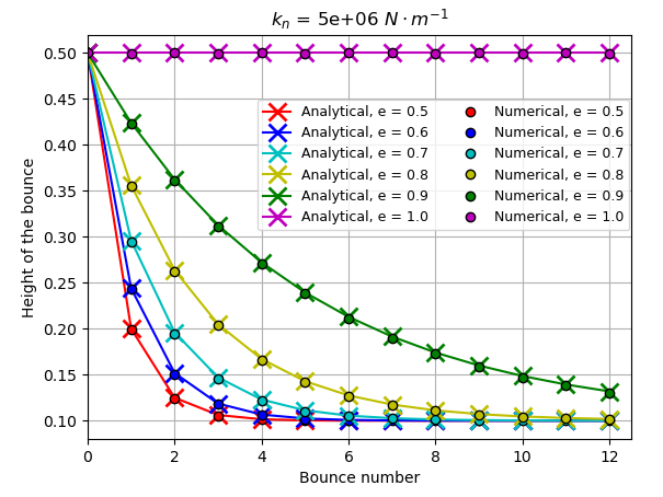
As the stiffness is increased, the agreement between the results obtained in the simulations and the analytical solution improves. This is due to the assumption of instantaneous contact, which becomes false for an elastic particle. Since the particle is less stiff, the contact time between the particle and the wall is longer, thus the damping term in the force calculation comes into effect over a longer period and more kinetic energy is lost.