Ribbon Mixer Using a Single Rotating Reference Frame#

When designing an industrial mixer, it is essential to evaluate the power consumed by the agitator. To do so, we usually refer to graphs correlating the power number ($N_p$) as a function of the Reynolds number ($Re$). $N_p$ is a dimensionless number that relates the power consumed by the agitator to the geometry of the system, the speed of the agitator, and the properties of the material being mixed (density $\rho$ and viscosity $\mu$). In this example, using a single rotating frame (SRF) model, we simulate a fluid being mixed in a double helical ribbon mixer for different flow conditions (different values of $Re$) to generate a numerical $N_p$ vs $Re$ curves.

In this example, we will be using the torque $(\Gamma \ [=] \ \text{N} \cdot \text{m})$ to calculate $N_p$ with the following expression:

\[N_p = \frac{2 \pi \Gamma}{\rho N^2 D^5}\]

where

$N$ is the angular velocity $[\text{rad} \cdot \text{s}^{-1}]$ of the agitator;
$D$ is the diameter of the impeller [m], and
$\rho$ is the density of the fluid $[\text{kg} \cdot \text{m}^{-3}]$.

Features#

Solver: lethe-fluid (with Q1-Q1)
Steady-state problem
Displays the use of a single rotating frame (srf) when modeling a complex rotating geometry
Calculation of the power number ($N_p$) using a python script
Use of a Digital Research Alliance of Canada (Alliance) cluster to run simulations

Files Used in This Example#

All files mentioned below are located in the example’s folder (examples/incompressible-flow/3d-ribbon-mixer-srf).

Bash script for gathering torques: Np_vs_Re/gather-torques.sh
Bash script for running simulations on a cluster (job script): Np_vs_Re/template/launch-mixer.sh
Experimental data file: Np_vs_Re/experimental.dat
Geometry file: diff-step-mesh.geo
Parameter file for $Re = 1$: Re1/ribbon-gls-Re1.prm
Parameter file for generating multiple cases: Np_vs_Re/ribbon-gls.prm
Postprocessing Python script for generating the $N_p$ vs $Re$ curves: Np_vs_Re/plot_Np_vs_Re.py
Python script for generating different cases: Np_vs_Re/template/lethe_case_generator.py
Python script for launching all the simulations on the cluster: Np_vs_Re/launch_all_mixers.py
STEP file: db-helical.step

Description of the Case#

We simulate the flow generated by a double helical ribbon impeller in a cylindrical mixing tank. The double helical ribbon impeller is a close-clearance impeller making it a great option for mixing viscous fluids.

The following figure represents the geometry of our system:

The dimensions of the system are listed in the following table:

Parameter	Description	Value
$T$	Tank diameter	$28.57$ cm
$H$	Tank height	$17.4625$ cm
$C$	Impeller off-bottom clearance	$T/4$
$D$	Impeller diameter	$27$ cm

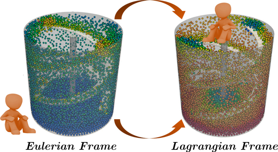
To simulate the flow in such complex geometry, we take advantage of the system’s symmetry and opt for a Lagrangian reference frame. Instead of observing the velocity profile from an Eulerian reference frame (or “lab reference frame”), we place ourselves on the impeller’s reference making it static and inducing a no-slip boundary condition. This way, the cylindrical tank will be the only moving geometry in our system. The figure below illustrates the difference between the Eulerian and Lagrangian reference frames [1].

Eulerian and Lagrangian reference frames

The rotating Lagrangian frame of reference is non-Galilean. Consequently, the Coriolis and the centrifugal forces must be added to the incompressible Navier-Stokes equations. The resulting set of equations is:

\[\begin{split}\nabla \cdot \mathbf{u} &= 0 \\ \frac{\partial \mathbf{u}}{\partial t} + \mathbf{u} \cdot \nabla \mathbf{u} &= -\frac{1}{\rho} \nabla p + \nu \nabla^2 \mathbf{u} +\mathbf{f} - \underbrace{\Omega \times \mathbf{u}}_{Coriolis} - \underbrace{\Omega \times (\mathbf{q} \times \mathbf{u})}_{Centrifugal}\end{split}\]

where $\mathbf{q}$ is the position in the fluid with respect to the center of rotation and $\mathbf{\Omega}$ is the angular velocity of the rotating reference frame. The Coriolis force adds a velocity dependent force to the Navier-Stokes equations whereas the centrifugal forces is independent of the flow and only modifies the pressure field.

In this example, we will start by simulating the case when $Re = 1$ and then follow with simulations for $Re$ values ranging from $0.1$ to $100$ to generate $N_p$ vs $Re$ curves.

The Reynolds number for our system is defined as follows:

\[Re = \frac{ND^2}{\nu}\]

where $\nu$ is the kinematic viscosity of the fluid $[\text{m}^2 \cdot \text{s}^{-1}]$.

Parameter File#

All subsections in ribbon-gls.prm except for velocity source were discussed in previous examples. However, the important sections are briefly explained for completeness.

Simulation Control#

subsection simulation control
    set method            = steady
    set output name       = mixer
    set output boundaries = true
    set output path       = ./output/
end

For this example, we consider that the regime is at a steady state, so we use a steady method. We set output boundaries = true to generate an auxiliary file that highlights the equipment walls by hiding the cells of the mesh. This allows a clearer visualization of the mixing setup.

Mesh#

subsection mesh
    set type      = gmsh
    set file name = diff-step-mesh.msh
    set simplex   = true
end

The type specifies the mesh format used, in this case, we have gmsh which corresponds to a file generated by Gmsh. The set file name command specifies the path to the file. In this case, we assume that the parameter and mesh files are in the same location. The .geo used to generate the gmsh mesh is also provided. It is also interesting to note that the .geo file used in the current example imports a CAD file (.step file) to get the double helical-shaped ribbon impeller.

Boundary Conditions#

subsection boundary conditions
  set number = 3
  subsection bc 0
    set id   = 1
    set type = function
    subsection u
      set Function expression = -10*y
    end
    subsection v
      set Function expression = 10*x
    end
    subsection w
      set Function expression = 0
    end
  end
  subsection bc 1
    set id   = 2
    set type = slip
  end

  subsection bc 2
    set id   = 3
    set type = noslip
  end
end

Three different boundary conditions are considered.

On the lateral walls and the bottom wall (id=1), we use the function boundary type. This type of boundary condition allows us to define the value of the velocity components using Function expression. We set $u = -10 \cdot y$, $v = 10 \cdot x$, and $w= 0$ to ensure that the impeller’s referential is static and the tank rotates in the opposite direction.
At the top of the vessel (id=2), a slip boundary condition is imposed on the free surface.
On the ribbon blades, a no-slip boundary condition applies (id=3).

The boundary conditions are described in the Boundary Conditions - CFD section of the documentation.

Physical Properties#

subsection physical properties
  subsection fluid 0
    set kinematic viscosity = 0.11602395351399172
   end
end

Here, the kinematic viscosity is set for a $Re = 1$, when the angular velocity is $10$ Hz and the diameter of the impeller is $0.27$ m.

Velocity Source#

subsection velocity source
    set rotating frame type    = srf
    set omega_z                = -10
end

In the velocity source subsection, we specify with rotating frame type = srf that we are in a single rotating reference frame. Since a centrifugal and a Coriolis force are induced by the rotating movement of the system, we are in a non-Galilean reference frame. These two additional force contributions must be taken into account in the Navier-Stokes equations and by setting the rotating frame type parameter to srf we do so. The omega_z parameter represents the angular velocity of the reference frame.

Forces#

The forces subsection controls the postprocessing of the torque and the forces acting on the boundaries of the domain.

subsection forces
    set verbosity             = verbose   # Output force and torques in log <quiet|verbose>
    set calculate torque      = true      # Enable torque calculation
    set torque name           = torque    # Name prefix of torque files
    set output precision      = 14        # Output precision
    set calculation frequency = 1         # Frequency of the force calculation
    set output frequency      = 1         # Frequency of file update
end

By setting calculate torque = true , the calculation of the torque resulting from the fluid dynamics physics on every boundary of the domain is automatically calculated. Setting verbosity = verbose will print out the value of the torque calculated. The output precision parameter holds the number of digits after the decimal point of the outputted value.

Non-linear Solver#

subsection non-linear solver
  subsection fluid dynamics
    set tolerance = 1e-10
  end
end

Lethe is an implicit CFD solver. Solving a steady-state problem requires the solution of a non-linear system of equations. By default, Lethe uses a Newton solver for which a tolerance must be specified. Here, we set our tolerance at 1e-10.

Linear Solver#

Relatively standard parameters are used for the linear solver. From our experience, the amg preconditioner is more robust and for that reason we will use it.

subsection linear solver
  subsection fluid dynamics
    set method                                    = gmres
    set max iters                                 = 100
    set relative residual                         = 1e-4
    set minimum residual                          = 1e-10
    set preconditioner                            = amg
    set amg preconditioner ilu fill               = 0
    set amg preconditioner ilu absolute tolerance = 1e-11
    set amg preconditioner ilu relative tolerance = 1.00
    set amg aggregation threshold                 = 1e-14  # Aggregation
    set amg n cycles                              = 2      # Number of AMG cycles
    set amg w cycles                              = false  # W cycles, otherwise V cycles
    set amg smoother sweeps                       = 2      # Sweeps
    set amg smoother overlap                      = 1      # Overlap
    set verbosity                                 = verbose
    set max krylov vectors                        = 500
  end
end

Running the Simulation#

Generating the Mesh#

Before launching the simulation, the mesh has to be generated. Using Gmsh, with the diff-step-mesh.geo file we generate the diff-step-mesh.msh file.

Assuming the gmsh executable is within your $PATH variable, you may generate the msh file by typing:

   gmsh -3 diff-step-mesh.geo -o diff-step-mesh.msh

You can then copy this file in the Re1 folder:

   cp diff-step-mesh.msh Re1

and then move it to the Np_vs_Re folder:

   mv diff-step-mesh.msh Np_vs_Re

Simulating for a Specific Flow Condition $(Re=1)$#

Launching the simulation is as simple as specifying the executable name and the parameter file. Assuming that the lethe-fluid executable is within your path, the simulation can be launched by typing:

  mpirun -np $number_of_CPUs lethe-fluid ribbon-gls-Re1.prm

Generating $N_p$ vs $Re$ Curves $(Re \in [0.1, 100])$#

To generate $N_p$ vs $Re$ curves, we are going to launch simulations for $25$ different values of $Re$. In this example, we will be launching these simulations on an Alliance cluster.

Generating the Different Cases#

Using lethe_case_generator.py, we generate the $25$ cases with $Re$ ranging from $0.1$ to $100$. Before running the Python script, it is important to specify your group account name, next to #SBATCH --account= among the job directives of the launch-mixer.sh script located in the template folder.

Warning

In order to run a job on an Alliance cluster, it is required to at least specify the time limit of the job (-- time) and your account (--account).

Here are a few examples of other job directives you may want to specify in your job script:

#!/bin/bash
#SBATCH --account=$yourgroupaccount
#SBATCH --time=1:00:00                  #maximum time for the simulation (hh:mm:ss or d-hh:mm:ss)
#SBATCH --ntasks-per-node=$X            #number of parallel tasks (as in mpirun -np X)
#SBATCH --nodes=1                       #number of whole nodes used (each with up to 40 tasks-per-node)
#SBATCH --mem=120G                      #memory usage per node. See cluster specification for maximal amount.
#SBATCH --job-name=$yourjobname
#SBATCH --mail-type=END                 #email preferences
#SBATCH --mail-type=FAIL
#SBATCH --mail-user=$your.email.adress@email.provider

Note

In this example, it is not necessary to specify the job name in the job script, we will be specifying it when submitting the jobs.

Warning

The cluster we used in this example was Béluga, you may need to adjust slightly the Bash script if you are going to run your simulations on a different cluster.

For our example, we will be running every job on $1$ node with $40$ tasks per node.

Once you have added your account and all the other job directives you wanted to add in the Bash script, we may generate the different cases by running the lethe_case_generator.py script. The kinematic viscosity for each $Re$ value, $\omega = 10 \ \text{Hz}$ and $D = 0.27 \ \text{m}$ is then calculated.

\[\nu = \frac{ND^2}{Re}\]

After that, the {{N}} expression in the Physical Properties subsection of the ribbon-gls.prm file is replaced by the calculated value of $\nu$ using the Jinja2 module. That is how the different .prm files for the different cases are generated.

Note

If you don’t have the Jinja2 module installed, you may install it using pip with the following command line:

  pip install Jinja2

After running the lethe_case_generator.py script you should have $25$ new folders named by the following syntax: mixer_$kinematic_viscosity_value. A new file named case_index.txt containing the names of all the new folders should also have been generated.

Copying Files to the Cluster#

We will now copy the Np_vs_Re folder to the cluster.

On your local computer, you may copy the Np_vs_Re folder to your scratch folder in the cluster with:

scp -r Path/To/Np_vs_Re username@clustername.computecanada.ca:/scratchPathInCluster

Tip

You may want to save the path to your scratch folder in the cluster in an environment variable on your local computer so that you do not have to type the long expression every time you copy files there. You may do so by adding the following line to your ~/.bashrc file (or any equivalent file) and sourcing the file:

export SCRATCH_PATH=username@clustername.computecanada.ca:/scratchPathInCluster

By doing so, you may copy the Np_vs_Re folder from your local computer with:

scp -r Path/To/Np_vs_Re $SCRATCH_PATH

Submitting Jobs and Launching Simulations#

The next step is to connect to an Alliance cluster:

ssh username@clustername.computecanada.ca

After connecting to your preferred cluster, you can submit your jobs by running the launch_all_mixers.py Python script located in the Np_vs_Re folder. After running the script, $25$ new jobs should have been generated. You may check if it is the case with the sq command. In the ST column of the output, you may see the status of each job. The two most common states are PD for pending or R for running.

Have trouble submitting the jobs?

If you are having issues with submitting the jobs please return to the Generating the Different Cases subsection and make sure that you added the required information in the launch-mixer.sh script.

Results and Discussion#

Simulating for a Specific Flow Condition $(Re=1)$#

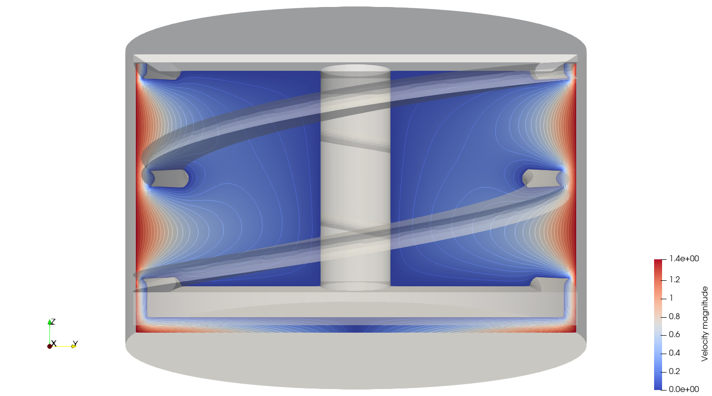
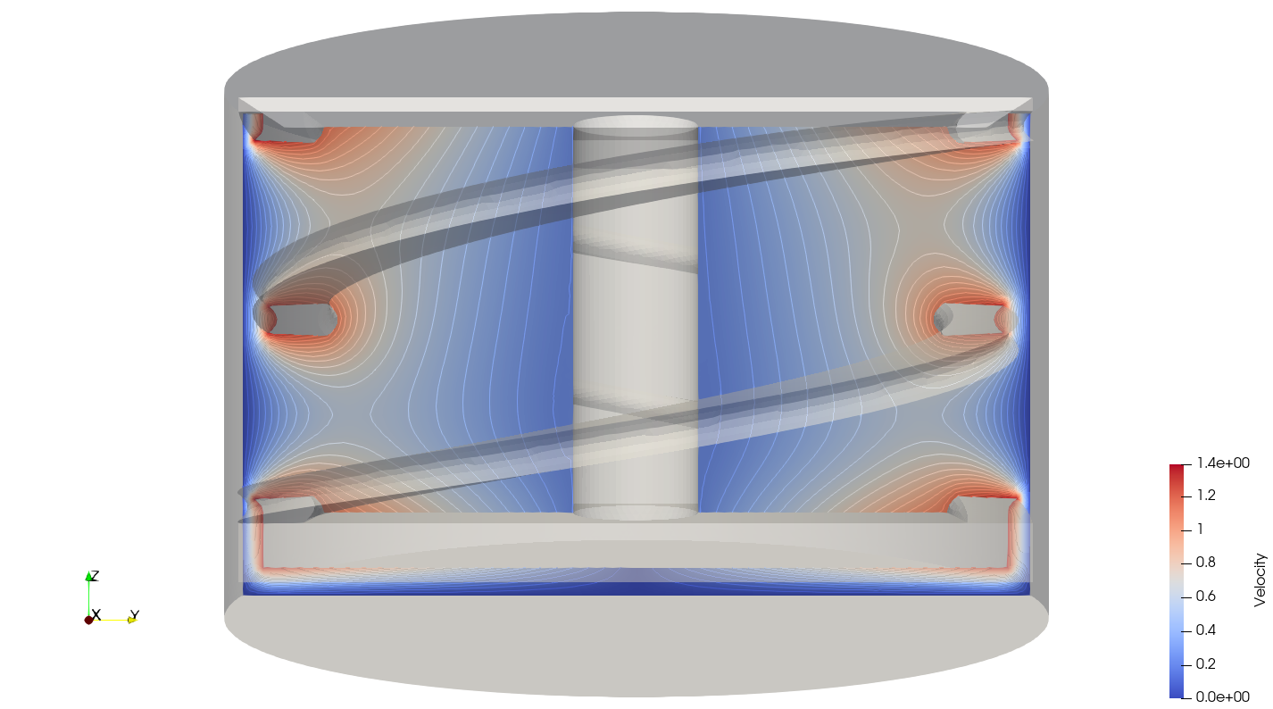
In the output subdirectory, you will find the mixer.pvd file that can be visualized using Paraview. In the figure below, the velocity magnitude are shown for a flow at $Re = 1$. Because a SRF is used, we can notice the rotational velocity imposed on the walls and the no-slip condition on the ribbon.

In the reference frame of the tank, the velocity field and its streamlines are visualized in an Eulerian frame. It is possible to do so by simply selecting velocity_eulerian in Paraview.

Ribbon Mixer Velocity in an Eulerian frame

Generating $N_p$ vs $Re$ Curves $(Re \in [0.1, 100])$#

Copying Files to Your Local Computer (Using SFTP)#

Before postprocessing the results of the simulations, you may want to copy the files from the remote machine to your local one. You may do so by connecting to the remote computer with the Secure File Transfer Protocol (SFTP):

sftp username@clustername.computecanada.ca

With the get command you may copy the remote Np_vs_Re folder:

get -r Path/To/Remote_Np_vs_Re Path/To/Local_directory

Note

Earlier, before launching the simulations, we could have also uploaded the initial Np_vs_Re folder using this method with the put command:

put -r Path/To/Local_Np_vs_Re Path/To/Remote_scratch_directory

Once the transfer is completed, you may exit with the exit command.

Postprocess Data#

In order to generate the $N_p$ vs $Re$ curves, we must first gather all the calculated $\Gamma$ from all different cases. You may do so by executing the gather-torques.sh Bash script. A new gather.dat file will be generated containing the number of cells and the $\Gamma$ components of each simulated case.

Note

In order to run the gather-torques.sh script, you must make sure that the script is executable. If it is not executable, you may add the permissions with:

chmod +x Path/To/gather-torques.sh

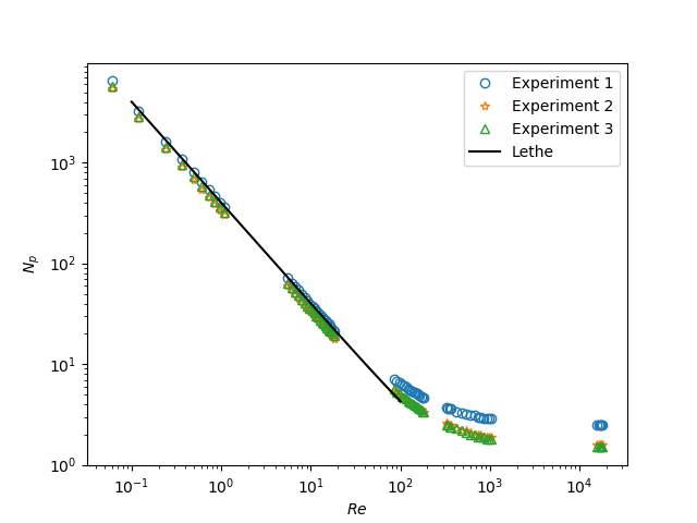
After that, you may run the plot_Np_vs_Re.py Python script to get the figure shown below.

As you can see, $N_p$ decreases when $Re$ increases. It is explained by:

\[N_p = \frac{2 \pi \Gamma}{\rho N^2 D^5} =\frac{1}{Re} \frac{2 \pi \Gamma}{\mu N D^3}\]

As we can see in the image above, for $Re < 100$ (laminar regime), the Lethe curve fits well with the experimental values.

Possibility for Extension#

It could be interesting to simulate at higher Reynolds numbers in a transient simulation and compare the results with the experimental data.

Parameter	Description	Value
\(T\)	Tank diameter	\(28.57\) cm
\(H\)	Tank height	\(17.4625\) cm
\(C\)	Impeller off-bottom clearance	\(T/4\)
\(D\)	Impeller diameter	\(27\) cm

Ribbon Mixer Using a Single Rotating Reference Frame#

Features#

Files Used in This Example#

Description of the Case#

Parameter File#

Simulation Control#

Mesh#

Boundary Conditions#

Physical Properties#

Velocity Source#

Forces#

Non-linear Solver#

Linear Solver#

Running the Simulation#

Generating the Mesh#

Simulating for a Specific Flow Condition \((Re=1)\)#

Generating \(N_p\) vs \(Re\) Curves \((Re \in [0.1, 100])\)#

Generating the Different Cases#

Copying Files to the Cluster#

Submitting Jobs and Launching Simulations#

Results and Discussion#

Simulating for a Specific Flow Condition \((Re=1)\)#

Generating \(N_p\) vs \(Re\) Curves \((Re \in [0.1, 100])\)#

Copying Files to Your Local Computer (Using SFTP)#

Postprocess Data#

Possibility for Extension#

Reference#