Non-Newtonian Flow past a Sphere#
This example showcases a laminar non-Newtonian flow around a sphere, with an a priori Reynolds number \(Re = 50\), using the Carreau rheological model.
Features#
Solvers:
lethe-fluid-sharp(with Q1-Q1)Steady-state problem
Non-Newtonian behavior
Ramping initial condition
Non-uniform mesh adaptation
Files Used in this Example#
Parameter file:
examples/sharp-immersed-boundary/sphere-carreau-with-sharp-interface/sphere-carreau-with-sharp-interface.prm
Description of the Case#
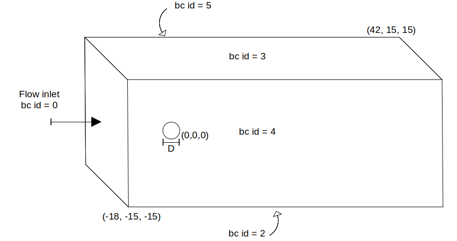
In this example, we study the flow around a static sphere using the sharp-interface method to represent the sphere. The geometry of the flow is the following, with a particle of diameter \(D = 1.0\) centered at \((0,0,0)\) and the flow domain located between \((-18,-15,-15)\) and \((42,15,15)\).
Parameter File#
Mesh#
The mesh is defined using the following subsection.
subsection mesh
  set type               = dealii
  set grid type          = subdivided_hyper_rectangle
  set grid arguments     = 2,1,1 : -18,-15,-15 : 42,15,15 : true
  set initial refinement = 4
end
The dimensions of the used domain are \((60 \times 30 \times 30)\), and the subdivided_hyper_rectangle is initially divided in \((2 \times 1 \times 1)\) cells, the cells are therefore cubic and of initial size \((30 \times 30 \times 30)\). Using set initial refinement = 4, the initial size of the cubic cells is \(30/2^4 = 1.875\). Since the particle size is small in regards to the mesh size, a refinement zone is generated around the particle to better capture it (see Box Refinement for more details).
subsection box refinement
  set number of refinement boxes = 1
  subsection box 0
    set additional refinement = 3
    subsection mesh
      set type           = dealii
      set grid type      = subdivided_hyper_rectangle
      set grid arguments = 1,1,1: -2,-2,-2 : 6,2,2 : true
    end
  end
end
Boundary Conditions#
We define the boundary conditions to have an inlet velocity of \(1~m/s\) on the left, slip boundary conditions parallel to the flow direction, and an outlet on the right of the domain.
subsection boundary conditions
  set number = 6
  subsection bc 0
    set id   = 0
    set type = function
    subsection u
      set Function expression = 1
    end
    subsection v
      set Function expression = 0
    end
    subsection w
      set Function expression = 0
    end
  end
  subsection bc 1
    set id   = 1
    set type = outlet
  end
  subsection bc 2
    set id   = 2
    set type = slip
  end
  subsection bc 3
    set id   = 3
    set type = slip
  end
  subsection bc 4
    set id   = 4
    set type = slip
  end
  subsection bc 5
    set id   = 5
    set type = slip
  end
end
Note
Since we use a deal.ii mesh, the boundary id = 1 is by default the second boundary in the x axis.
Physical Properties#
This example showcases a shear-thinning flow, for which the kinematic viscosity decreases when the local shear rate increases. The Carreau model is used. For more information on rheological models, see Physical Properties.
subsection physical properties
  set number of fluids = 1
  subsection fluid 0
    set rheological model = carreau
    subsection non newtonian
      subsection carreau
        set viscosity_0   = 0.063403
        set viscosity_inf = 0
        set lambda        = 10
        set a             = 2.0
        set n             = 0.5
      end
    end
  end
end
With viscosity_inf = 0 (3-parameter Carreau model), the a priori Reynolds number can be estimated using :
We use an a priori Reynolds number, since it is not possible, a priori, to know the effective kinematic viscosity of the flow. For the given parameters, the a priori Reynolds number is \(50\).
Initial Conditions#
This example uses a ramping initial condition that first ramps on the n parameter, and then on the viscosity_0 parameter. This allows for a smooth transition of non-Newtonian behavior level and regime.
subsection initial conditions
  set type = ramp
  subsection ramp
    subsection n
      set initial n  = 1.0
      set iterations = 2
      set alpha      = 0.5
    end
    subsection kinematic viscosity
      set initial kinematic viscosity = 1.0
      set iterations                  = 2
      set alpha                       = 0.5
    end
  end
end
The first initial condition simulation solves for n=1.0, viscosity_0 = 1.0, viscosity_inf = 0, lambda=10 and a=2. The subsequent initial simulations are:
(Second
niteration)n=0.75,viscosity_0 = 1.0,viscosity_inf = 0,lambda=10anda=2;(First
kinematic viscosityiteration)n=0.5,viscosity_0 = 1.0,viscosity_inf = 0,lambda=10anda=2;(Second
kinematic viscosityiteration)n=0.5,viscosity_0 = 0.531702,viscosity_inf = 0,lambda=10anda=2
and the first simulation uses the parameters in the subsection physical properties. For more information on ramping initial conditions, see Initial Conditions.
Particle#
In this case, we want to define a spherical boundary of radius \(0.5\), with its center at \((0,0,0)\) and that has no velocity. For more information on particle immersed boundary conditions using a sharp interface, see Sharp-Immersed-Boundary.
subsection particles
  set number of particles                     = 1
  set assemble Navier-Stokes inside particles = false
  subsection extrapolation function
    set stencil degree = 2
    set length ratio  = 1
  end
  subsection local mesh refinement
    set initial refinement                = 2
    set refine mesh inside radius factor  = 0.85
    set refine mesh outside radius factor = 1.3
  end
  subsection particle info 0
    set type             = sphere
    set shape arguments  = 0.5
    subsection position
      set Function expression = 0;0;0
    end
  end
end
The hypershell around the boundary between refine mesh inside radius factor (\(r = 0.425\)) and refine mesh outside radius factor (\(r = 0.65\)) will initially be refined twice (initial refinement = 2).
Simulation Control#
The simulation is solved at steady-state with 2 mesh adaptations.
subsection simulation control
  set method            = steady
  set number mesh adapt = 2
  set output name       = sharp-carreau-output
  set output frequency  = 1
  set subdivision       = 1
end
Mesh Adaptation#
To generate an additional refinement zone around the immersed boundary, the mesh adaptation type must be set to adaptive. During both of the mesh refinement steps, \(40\%\) of the cells with be split in \(8\) (fraction refinement = 0.4) using a velocity-gradient Kelly operator.
subsection mesh adaptation
  set type                 = adaptive
  set error estimator      = kelly
  set fraction coarsening  = 0.1
  set fraction refinement  = 0.4
  set fraction type        = number
  set frequency            = 1
  set max number elements  = 8000000
  set min refinement level = 0
  set max refinement level = 11
  set variable             = velocity
end
Results#
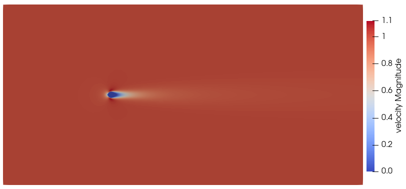
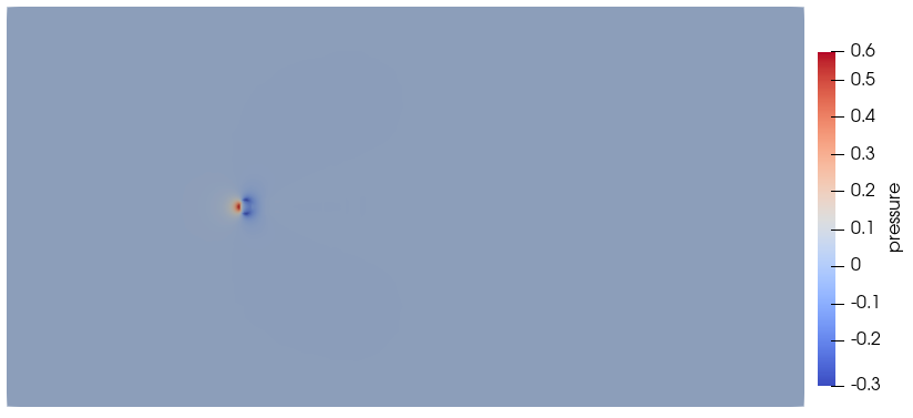
Using Paraview, the steady-state velocity profile and the pressure profile can be visualized by operating a slice along the xy-plane (z-normal) that cuts in the middle of the sphere (See documentation).
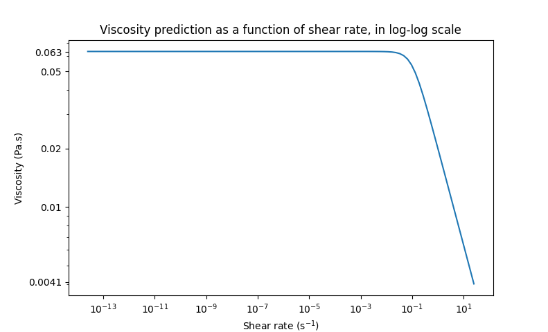
We can also see the kinematic viscosity profile throughout the domain, that is a function of the shear rate magnitude profile. Close to the particle, the shear rate is high which decreases the kinematic viscosity.
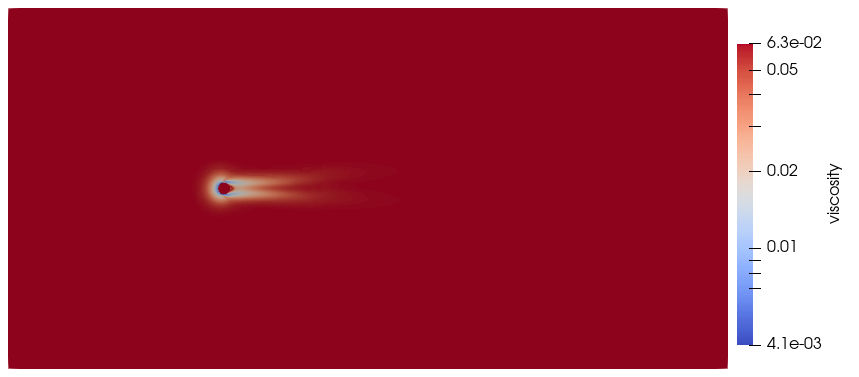
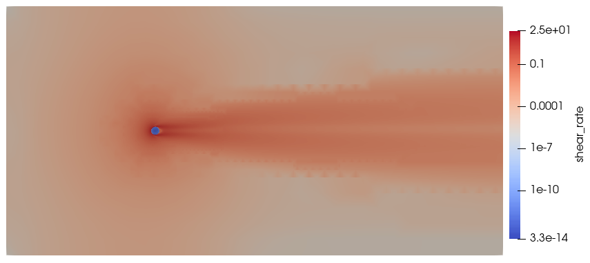
We can notice that the kinematic viscosity rapidly reaches a plateau at \(\eta=0.063\). Given the parameters in the subsection physical properties, the kinematic viscosity behavior should be given by:
We get the following torques and forces applied on the particle for each of the mesh refinements. The drag force applied on the particle is the effective force in the same direction as the flow, which is in the \(x\) direction in this case.
particle_ID    T_x      T_y       T_z      f_x       f_y       f_z      f_xv     f_yv      f_zv     f_xp      f_yp      f_zp
        0   -0.000010 0.000019 -0.000041 0.412175  0.000036  0.000026 0.143775 0.000036  0.000026 0.268400  0.000000  0.000000
        0   -0.000000 0.000001 -0.000007 0.415760  0.000006 -0.000001 0.162430 0.000006 -0.000001 0.253330 -0.000000 -0.000000
        0   -0.000000 0.000000 -0.000001 0.424786 -0.000002 -0.000002 0.176205 0.000001 -0.000000 0.248581 -0.000002 -0.000001
Note
Because this analysis concerns non-Newtonian flow, there is no known solution for the drag coefficient. For a Newtonian flow at \(Re = 50\), the drag force would be \(0.6165\). Therefore, the drag force was decreased using a shear-thinning fluid.
Possibilities for Extension#
High-order methods : Lethe supports higher order interpolation. This can yield much better results with an equal number of degrees of freedom than traditional second-order (Q1-Q1) methods, especially at higher Reynolds numbers.
Reynolds number : By changing the inlet velocity, it can be interesting to see the impact of the shear-thinning behavior on the effective drag force.
Non-Newtonian parameters : It can also be interesting to change the Carreau model parameters, i.e. changing the slope to appreciate the behavior change.
Note
The Carreau model is limited to shear-thinning flows. For shear-thickening models (e.g., the power-law model), we refer the reader to Physical Properties.