Taylor-Couette Flow

This example showcases another classical fluid mechanics problem, the Taylor-Couette flow [1]. This example introduces the usage of analytical solution and monitors the convergence of the CFD solver by using progressively refined meshes.

Features

• Solvers: lethe-fluid (with Q1-Q1 and Q2-Q1) or lethe-fluid-block (with Q2-Q1)

• Steady-state problem

• Displays the use of the analytical solution to calculate the mesh convergence

• Displays the calculation of the torque induced by the fluid on a boundary

Files Used in This Example

All files mentioned below are located in the example’s folder (examples/incompressible-flow/2d-taylor-couette).

• Parameter file: taylor-couette.prm

• Postprocessing Python script: postprocess_taylor_couette.py

Description of the Case

Taylor-Couette flow is a fluid flow in the gap between two long concentric cylinders with different rotational velocities. One or both of these cylinders may rotate along the axis, however generally it is assumed that the outer cylinder is fixed, and the inner cylinder rotates with a constant angular velocity. For the Taylor-Couette flow, an analytical solution of the Navier-Stokes equations can be found, although this solution is not stable for all ranges of operating conditions and becomes unstable at high Reynolds number.

We assume that the inner cylinder rotates at a constant angular velocity \(\omega\) in the anti-clockwise direction, while the outer cylinder is fixed. The following figure shows the geometry of this problem and the corresponding boundary conditions:

The analytical solution of this problem can be found relatively easily in cylindrical coordinates (see for example the book by Bird, Stewart and Lightfoot [1]):

\[u_{\theta} = \omega R \kappa \frac{\left ( \frac{R}{r} - \frac{r}{R} \right )} {\left( \frac{1}{\kappa} - \kappa \right)}\]

where \(u_{\theta}\) is the angular velocity, \(R\) is the radius of the outer cylinder, \(\kappa\) takes a value between 0 and 1.0 and represents the ratio between the radius of the inner cylinder and the radius of the outer cylinder (\(\kappa=R_{i}/ R\)) and \(r\) is the radial position. Since the simulation in Lethe is in Cartesian coordinates, this analytical solution will have to be converted to Cartesian coordinates to be usable. As we shall see, this is not as hard as it seems. Interestingly, this flow also possesses an analytical solution for the torque \(T_z\) acting on the inner cylinder:

\[T_z = 4 \pi \mu \omega R^2 L \frac{\kappa^2}{1-\kappa^2}\]

where \(\mu\) is the dynamic viscosity and \(L\) is the height of the cylinder. Since we simulate the problem in 2D, we assume that \(L=1\) without loss of generality.

Parameter File

We first establish the mesh used for the simulation

Mesh

The mesh subsection specifies the computational grid:

subsection mesh
  set type               = dealii
  set grid type          = hyper_shell
  set grid arguments     = 0, 0 : 0.25 : 1 : 4:  true
  set initial refinement = 3
end

The type specifies the mesh format used. We use the hyper_shell mesh generated from the deal.II GridGenerator . This GridGenerator generates the mesh of the interstice between two concentric cylinder. The arguments of this grid type are the position of center of the cylinders (0, 0), the inner cylinder radius (0.25), the outer cylinder radius (1) and the number of subdivision in the azimuthal direction (4). All arguments are separated by :. We set colorize=true and this sets the boundary ID of the inner cylinder to 0 and of the outer cylinder to 1.

The last parameter specifies the initial refinement of the grid. Most deal.II grid generators contain a minimal number of cells. The hyper_shell mesh is made of four cells. Indicating an initial refinement=3 implies that the initial mesh is refined 3 times. In 2D, each cell is divided by 4 per refinement. Consequently, the final grid is made of 256 cells.

Boundary Conditions

The boundary conditions subsection establishes the constraints on different parts of the domain:

subsection boundary conditions
  set number = 2
  subsection bc 0
    set type = function
    subsection u
      set Function expression = -y
    end
    subsection v
      set Function expression = x
    end
    subsection w
      set Function expression = 0
    end
  end
  subsection bc 1
    set type = noslip
  end
end

First, the number of boundary conditions to be applied must be specified. For each boundary condition, the id of the boundary as well as its type must be specified. The outer cylinder (1) is static and, consequently, a noslip boundary condition is applied. The inner cylinder is rotating at a constant angular velocity (\(\omega=1\)). To impose this boundary condition, we use the type=function and prescribe a function for the components of the velocity (remembering that \(\mathbf{u}=[u,v]^T\)). By prescribing \(\mathbf{u}=[-y,x]^T\), we prescribe the rotation of the inner cylinder at an angular velocity of \(1 \ \text{rad/s}\) in the trigonometric direction.

Physical Properties

The analytical solution for the Taylor-Couette problem is only valid at low Reynolds number. We thus set the kinematic viscosity to 1.

subsection physical properties
  subsection fluid 0
    set kinematic viscosity = 1.0
  end
end

FEM Interpolation

Lethe supports the use of arbitrary interpolation order. The \(\mathcal{L}^2\) norm of the error is \(\mathcal{O}\left(h^{n+1} \right)\) where \(h\) is a measure of the element size and \(n\) is the interpolation order of the velocity. However, since the torque applied on the inner cylinder depends on the deviatoric stress tensor, which depends on the velocity gradient, its error will be \(\mathcal{O}(h^n)\). Taking this into account, we use second order polynomials in this example to obtain higher accuracy on the torque. We specify the interpolation order for both pressure and velocity using the FEM subsection:

subsection FEM
    set velocity order = 2
    set pressure order = 1
end

Note

With the lethe-fluid solver, Q2-Q2 elements could also be used. However, we have not found that these lead to better results when the flows are at a low Reynolds number.

Analytical Solution

To monitor the convergence of the CFD solver, we can provide Lethe with an expression for the analytical expression of the velocity field. Using this expression and the velocity field obtained from the solver, Lethe will calculate the \(\mathcal{L}^2\) norm of the error. The \(L^2\) norm of the error is calculated as:

\[L^2 = \int_\Omega (u-u_a)^2 \mathrm{d} \Omega\]

where \(u\) is the numerical solution, \(u_a\) is the analytical solution and \(\Omega\) is the domain of the simulation.

subsection analytical solution
  set enable = true
  subsection uvwp
    # A= -(kappa * kappa) / (1. - kappa * kappa);
    # B= ri * ri / (1. - kappa * kappa);
    set Function constants  = kappa=0.25, ri=0.25, A=-0.06666666666666667, B=0.06666666666666666667
    set Function expression = -sin(atan2(y,x))*(-(kappa*kappa) / (1-kappa*kappa)* sqrt(x*x+y*y)+ ri*ri/(1-kappa*kappa)/sqrt(x*x+y*y)); cos(atan2(y,x))*(-(kappa*kappa) / (1-kappa*kappa)* sqrt(x*x+y*y)+ ri*ri/(1-kappa*kappa)/sqrt(x*x+y*y)) ; A*A*(x^2+y^2)/2 + 2 *A*B *ln(sqrt(x^2+y^2)) - 0.5*B*B/(x^2+y^2)
  end
end

To monitor the error in a simulation, we must set enable = true. We must convert the analytical solution from cylindrical coordinates to Cartesian and this is why the resulting Function expression is slightly barbaric. Notably, this explains why we often see the occurrence of the term sqrt(x^2+y^2) which is in fact the radius \(r=\sqrt{x^2+y^2}\).

Simulation Control

The simulation control subsection controls the flow of the simulation. Two additional parameters are introduced in this example. By setting number mesh adapt = 3 we configure the simulation to solve the fluid dynamics on the mesh and on two subsequently refined meshes. This approach is very interesting, because the solution on the coarse mesh also serves as the initial guest for the solution on the finer mesh. We set subdivision = 2 to allow the rendering of high-order elements in Paraview. This will be explained later in the example.

subsection simulation control
  set method            = steady
  set output name       = couette
  set subdivision       = 2
  set number mesh adapt = 3 # time-stepping method must be "steady"
end

Mesh Adaptation

Mesh adaptation is quite complex in Lethe. The mesh can be dynamically adapted using Kelly error estimates on the velocity, pressure or variables arising from other physics. Lethe also supports uniform mesh refinement. Since we wish to measure the convergence of the error with respect to an analytical solution, we specify a uniform mesh refinement by setting type = uniform

subsection mesh adaptation
  set type = uniform
end

Forces

The forces subsection controls the postprocessing of the torque and the forces acting on the boundaries of the domain.

subsection forces
  set verbosity        = verbose # Output force and torques in log <quiet|verbose>
  set calculate torque = true    # Enable torque calculation
end

By setting calculate torque = true, the calculation of the torque resulting from the fluid dynamics physics on every boundary of the domain is automatically calculated. Setting verbosity = verbose will print out the value of the torque calculated for each mesh.

Rest of the Subsections

The non-linear solver and linear solver subsections do not contain any new information in this example.

Running the Simulation

Launching the simulation is as simple as specifying the executable name and the parameter file. Assuming that the lethe-fluid executable is within your path, the simulation can be launched by typing:

lethe-fluid taylor-couette.prm

Lethe will generate a number of files. The most important one bears the extension .pvd. It can be read by visualization programs such as Paraview.

Results and Discussion

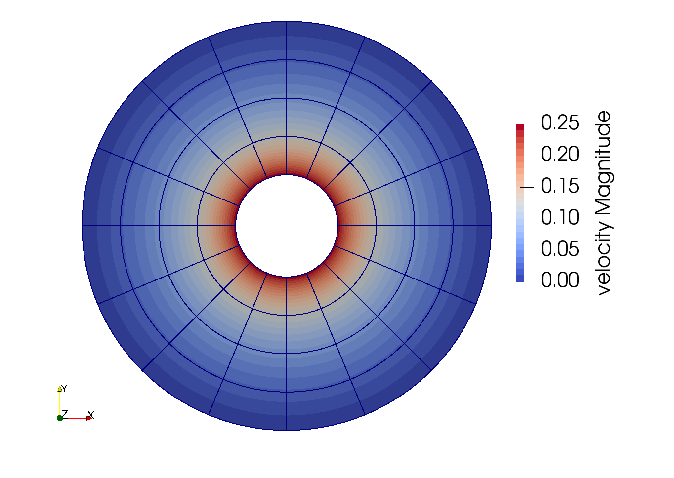
Using Paraview, the steady-state velocity profile can be visualized:

As it can be seen, each cell is curved because a Q2 isoparametric mapping was used. To visualize these high-order cells, we need to subdivide the regular cell to store additional information onto them. A good practice is to use as many subdivisions as the interpolation order of the scheme. Hence, we used subdivision = 2 in the simulation control subsection. Finally, by default, Paraview does not render high-order elements. To enable the rendering of high-order elements, the Nonlinear Subdivision Level slider must be increased above one. For more information on this topic, please consult the deal.II wiki page on rendering high-order elements.

Note

To showcase the curvature of the cells, we have illustrated the results on a mesh coarser that the initial mesh used in this simulation.

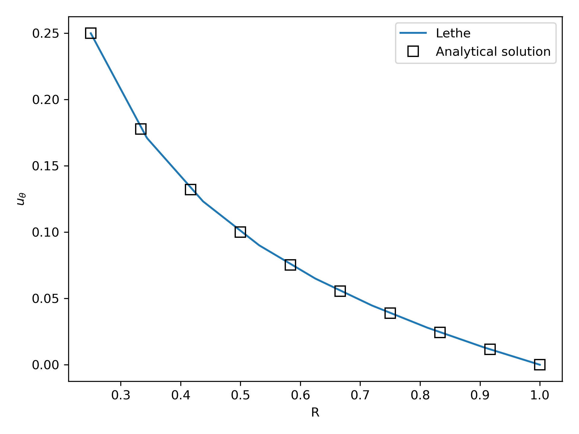
A python script provided in the example folder allows to compare the velocity profile along the radius with the analytical solution. Using this script, the following resuts are obtained for the initial mesh:

The end of the simulation log provides the following information about the convergence of the error:

cells  error_velocity    error_pressure
  256 9.623524e-05    - 2.595531e-04    -
 1024 1.270925e-05 2.92 6.696872e-05 1.95
 4096 1.613718e-06 2.98 1.675237e-05 2.00
16384 2.025381e-07 2.99 4.181523e-06 2.00

This table reports the \(\mathcal{L}^2\) norm of the error as a function of the number of cells. The third and the fifth column report the apparent order of convergence of the scheme. We see that the velocity converges at third order and the pressure at second order. This is exactly what is expected when using Q2-Q1 elements.

Note

A curious reader will find that very similar results are obtained when using Q2-Q2 elements. For flows at low Reynolds number, using equal order elements for the pressure does not lead to a higher convergence rate.

Finally, the simulation produces a file that contains the torque calculated on every boundary. The file torque.00.dat contains the torque on bc 0 and the file torque.01.dat contains the torque on bc 1.

For the boundary 0, the following torques are obtained:

cells     T_x          T_y           T_z
256   0.0000000000 0.0000000000 -0.8192063151
1024  0.0000000000 0.0000000000 -0.8319958810
4096  0.0000000000 0.0000000000 -0.8361362739
16384 0.0000000000 0.0000000000 -0.8373265692

For the boundary 1, the following torques are obtained:

 cells     T_x          T_y          T_z
  256 0.0000000000 0.0000000000 0.8357077079
 1024 0.0000000000 0.0000000000 0.8372702342
 4096 0.0000000000 0.0000000000 0.8376393911
16384 0.0000000000 0.0000000000 0.8377288180

The analytical value of the torque is : \(T_z=0.837758\). Two main conclusions can be drawn. First, the torque obtained from the simulation on both boundaries converges to the analytical solution (at a second-order rate). Secondly, the torque on the difference between the torque on the outer and the inner cylinder converges to zero. This is what we would expect due to Newton’s third law (action-reaction). However, it is only reached once the mesh is sufficiently fine and we note a significant (\(\approx 2\%\)) disagreement between the two torques for the coarsest mesh.

Possibilities for Extension

• Calculate the order of convergence for the torque \(T_z\).

• It could be very interesting to investigate this flow in 3D at a higher Reynolds number to see the apparition of the Taylor-Couette instability. This, however, would be a major undertaking.

References

[1]

R. B. Bird, W. E. Stewart, and E. N. Lightfoot, Transport Phenomena, vol. 1. John Wiley & Sons, 2006.