Taylor-Green Vortex

This example showcases another canonical fluid mechanics problem: the Taylor-Green vortex. This example features both the traditional matrix-based solver within Lethe (lethe-fluid) and the matrix-free solver (lethe-fluid-matrix-free) which is more computationally efficient, especially for high-order elements (Q2 and above). Postprocessing capabilities for enstrophy and kinetic energy are also demonstrated.

Features

• Solvers: lethe-fluid (with Q2-Q2) or lethe-fluid-matrix-free (with Q2-Q2 or Q3-Q3)

• Transient problem using bdf3 time integrator

• Displays the calculation of enstrophy and total kinetic energy

Files Used in This Example

All files mentioned below are located in the example’s folder (examples/incompressible-flow/3d-taylor-green-vortex).

• Parameter files: tgv-matrix-based.prm and tgv-matrix-free.prm

• Postprocessing Python scripts: plot_dissipation_rate.py and calculate_dissipation_rate.py

Description of the Case

The Taylor–Green vortex is an unsteady flow of a decaying vortex, which has an exact closed form solution of the incompressible Navier–Stokes equations in Cartesian coordinates. It is named after the British physicist and mathematician Geoffrey Ingram Taylor and his collaborator A. E. Green [1]. In the present case, we simulate one Taylor-Green vortex at a Reynolds number of 1600 in a domain \(\Omega = [-\pi,\pi]\times[-\pi,\pi]\times[-\pi,\pi]\) using periodic boundary conditions.

The three velocity components \([u_x,u_y,u_z]^T\) and the pressure \(p\) are specified at time \(t=0\) by:

\[\begin{split}u_{x} &= \sin(x)*\cos(y)*\cos(z) \\ u_{y} &= -\cos(x)*\sin(y)*\cos(z)\\ u_{z} &= 0 \\ p &= \frac{1}{16}*\left[\cos(2x)+\cos(2y)\right]\left[\cos(2z)+2\right]\end{split}\]

In this case, the vortex, which is initially 2D, will decay by generating smaller 3D turbulent structures (vortex tubes, rings and sheets). This decay can be monitored through the total kinetic energy of the system. Since the simulation domain is periodic, it can be demontrated that the time derative of the total kinetic energy \(E_\mathrm{k}\) is directly related to the enstrophy \(\mathcal{E}\) such that:

\[\begin{split}\frac{\mathrm{d}E_\mathrm{k}}{\mathrm{d}t} &= -\mathcal{E} \\ E_k &= \frac{1}{\Omega} \int_{\Omega} \frac{\mathbf{u}\cdot \mathbf{u}}{2} \mathrm{d}\Omega \\ \mathcal{E} &= \frac{1}{\Omega} \int_{\Omega} \frac{\mathbf{\omega}\cdot \mathbf{\omega}}{2} \mathrm{d}\Omega\end{split}\]

where \(\mathbf{\omega}=\nabla \times \mathbf{u}\) is the vorticity. The results we obtain are compared to reference spectral results extracted from Wang et al. [2].

Parameter File

Mesh

The mesh subsection specifies the computational grid:

subsection mesh
  set type               = dealii
  set grid type          = hyper_cube
  set grid arguments     = -3.14159265359 : 3.14159265359 : true
  set initial refinement = 5
end

The type specifies the mesh format used. We use the hyper_cube mesh generated from the deal.II GridGenerator . We set colorize = true to be able to adequately set-up the periodic boundary conditions.

The last parameter specifies the initial refinement of the grid. Indicating an initial refinement = 5 implies that the initial mesh is refined 5 times. In 3D, each cell is divided by 8 per refinement. Consequently, the final grid is made of 32768 cells.

Boundary Conditions

The boundary conditions subsection establishes the constraints on different parts of the domain:

subsection boundary conditions
  set number = 3
  subsection bc 0
    set type               = periodic
    set id                 = 0
    set periodic_id        = 1
    set periodic_direction = 0
  end
  subsection bc 1
    set type               = periodic
    set id                 = 2
    set periodic_id        = 3
    set periodic_direction = 1
  end
  subsection bc 2
    set type               = periodic
    set id                 = 4
    set periodic_id        = 5
    set periodic_direction = 2
  end
end

First, the number of boundary conditions to be applied must be specified. For each boundary condition, the id of the boundary as well as its type must be specified. All boundaries are periodic. The x- (id=0) is periodic with the x+ boundary (id=1), the y- (id=2) is periodic with the y+ boundary (id=3) and so on and so forth. For each periodic boundary condition, the periodic direction must be specified. A periodic direction of 0 implies that the normal direction of the wall is the \(\mathbf{e}_x\) vector, 1 implies that it’s the \(\mathbf{e}_y\).

Physical Properties

The Reynolds number of 1600 is set solely using the kinematic viscosity since the reference velocity is one:

subsection physical properties
  set number of fluids = 1
  subsection fluid 0
    set kinematic viscosity = 0.000625
  end
end

FEM Interpolation

The results obtained for the Taylor-Green vortex are highly dependent on the numerical dissipation that occurs within the CFD scheme. Generally, high-order methods outperform traditional second-order accurate methods for this type of flow. In the present case, we will investigate the usage of both second and third degree polynomial.

subsection FEM
    set velocity order = 2 #3 for Q3
    set pressure order = 2 #3 for Q3
end

Post-processing

subsection post-processing
  set verbosity                = verbose
  set calculate enstrophy      = true
  set calculate kinetic energy = true
end

To monitor the kinetic energy and the enstrophy, we set both calculation to true in the post-processing section.

Simulation Control

The simulation control subsection controls the flow of the simulation. To maximize the temporal accuracy of the simulation, we use a third order bdf3 scheme. Results are written every 2 time-steps. To ensure a more adequate visualization of the high-order elements, we set subdivision = 3. This will allow Paraview to render the high-order solutions with more fidelity.

subsection simulation control
  set method            = bdf3
  set time step         = 0.05
  set number mesh adapt = 0
  set time end          = 20
  set output frequency  = 2
  set subdivision       = 3
end

Matrix-based - Non-linear Solver

The calculation of the Jacobian matrix is expensive when using high-order elements. In transient simulations such as this one, it can be desirable to minimize the amount of time this matrix is calculated. To achieve this, we use the inexact_newton non-linear solver which reuses the Jacobian matrix as long as it is sufficiently valid.

subsection non-linear solver
  subsection fluid dynamics
    set solver            = inexact_newton
    set verbosity         = verbose
    set tolerance         = 1e-3
    set reuse matrix      = true
    set matrix tolerance  = 0.01
  end
end

Matrix-based - Linear Solver

Since this is a transient problem, the linear solver can be relatively simple. We use the GMRES iterative solver with ILU preconditioning and a low fill level of 0.

subsection linear solver
  subsection fluid dynamics
    set verbosity                             = verbose
    set method                                = gmres
    set max iters                             = 200
    set max krylov vectors                    = 200
    set relative residual                     = 1e-4
    set minimum residual                      = 1e-12
    set ilu preconditioner fill               = 0
    set ilu preconditioner absolute tolerance = 1e-12
    set ilu preconditioner relative tolerance = 1.00
  end
end

Matrix-free - Non-linear Solver

The non-linear solver used in the matrix-free solver is straightforward. We use Newton’s method with a tolerance of \(10^{-3}\).

subsection non-linear solver
  subsection fluid dynamics
    set tolerance = 1e-3
    set verbosity = verbose
  end
end

Matrix-free - Linear Solver

The lethe-fluid-matrix-free has significantly more parameters for its linear solver. The new parameters are all related to the geometric multigrid preconditioner that is used by the matrix-free algorithm.

subsection linear solver
  subsection fluid dynamics
    set method            = gmres
    set max iters         = 100
    set relative residual = 1e-4
    set minimum residual  = 1e-7
    set preconditioner    = gcmg
    set verbosity         = verbos

    # MG parameters
    set mg verbosity       = quiet
    set mg min level       = -1
    set mg level min cells = 16

    # Smoother
    set mg smoother iterations     = 10
    set mg smoother eig estimation = true

    # Eigenvalue estimation parameters
    set eig estimation smoothing range = 5
    set eig estimation cg n iterations = 20
    set eig estimation verbosity       = verbose

    # Coarse-grid solver
    set mg coarse grid solver                 = gmres
    set mg gmres max iterations               = 2000
    set mg gmres tolerance                    = 1e-7
    set mg gmres reduce                       = 1e-4
    set mg gmres max krylov vectors           = 30
    set mg gmres preconditioner               = ilu
    set ilu preconditioner fill               = 1
    set ilu preconditioner absolute tolerance = 1e-10
    set ilu preconditioner relative tolerance = 1.00
  end
end

We set mg verbosity = quiet to prevent logging of the multigrid parameters during the simulation. Setting mg min level = -1 ensures that the mg level min cells = 16 parameter is used to determine the coarsest level. It is important to ensure that the Taylor-Green vortex has sufficient cells on the coarsest level since periodic boundary conditions are used. Indeed, using a coarsest level with a single cell can lead to a problematic situation where too few degrees of freedom are available on the coarsest level.

The smoother, Eigenvalue estimation parameters and coarse-grid solver subsections are explained in the Theory Guide (under construction).

Running the Simulation

Launching the simulation is as simple as specifying the executable name and the parameter file. Assuming that the lethe-fluid or lethe-fluid-matrix-free executables are within your path, the matrix-based simulation scan be launched by typing:

mpirun -np n_proc lethe-fluid tgv-matrix-based.prm

and the matrix-free simulations can be launched by typing

mpirun -np n_proc lethe-fluid-matrix-free tgv-matrix-free.prm

For a 5 initial refinements (\(32^3\) Q2 cells), the matrix-based solver takes around 1 hour and 20 minutes on 16 cores while the matrix-free solver takes less than 20 minutes. Running the same problem, but in Q3 (\(32^3\) Q3 cells), the matrix-free solver takes less than 2 hours while the matrix-based solver takes close to a day and consumes a tremendous amount of ram (approx. 80 GB). If you have 64 GB of ram, you can run an even finer mesh (\(64^3\) Q3 cells) using the matrix-free solver in approximately 16 hours.

Results and Discussion

The flow patterns generated by the Taylor-Green vortex are quite complex. The following animation displays the evolution of velocity iso-contours as the vortex break downs and generates smaller structures.

Using the enstrophy.dat and kinetic_energy.dat files generated by Lethe, the temporal decay of the kinetic energy can be monitored. First, we calculate the time-derivative of the kinetic energy by invoking the first script present in the example folder:

python3 calculate_dissipation_rate.py -i kinetic_energy.dat -o output.dat

Then, by invoking the second script present in the example, a plot comparing the kinetic energy decay with the enstrophy is generated:

python3 plot_dissipation_rate.py -ke kinetic_energy_decay.dat -ens enstrophy.dat -v 0.000625

Tip

A nice plot with a zoomed in section can be generated by adding the argument -z True to the command above.

The following plot shows the decay of kinetic energy as measured.

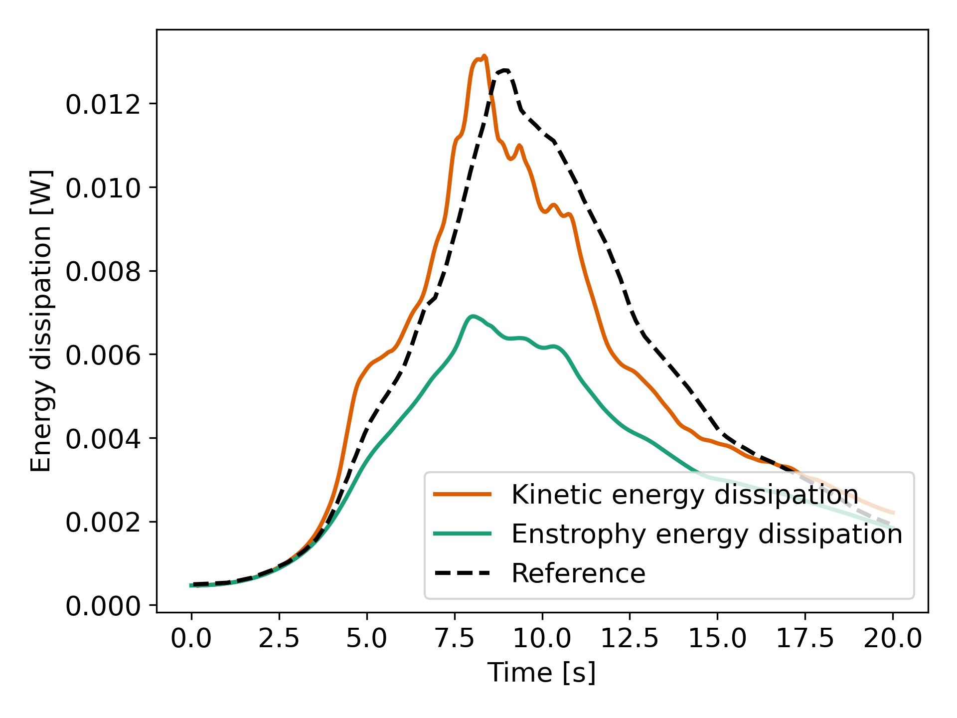
We note that the kinetic energy decay does not match that of the reference, but also that there is significant numerical dissipation since the enstrophy does not match the kinetic energy decay. Increasing the order from Q2 to Q3 yield the following results which are better:

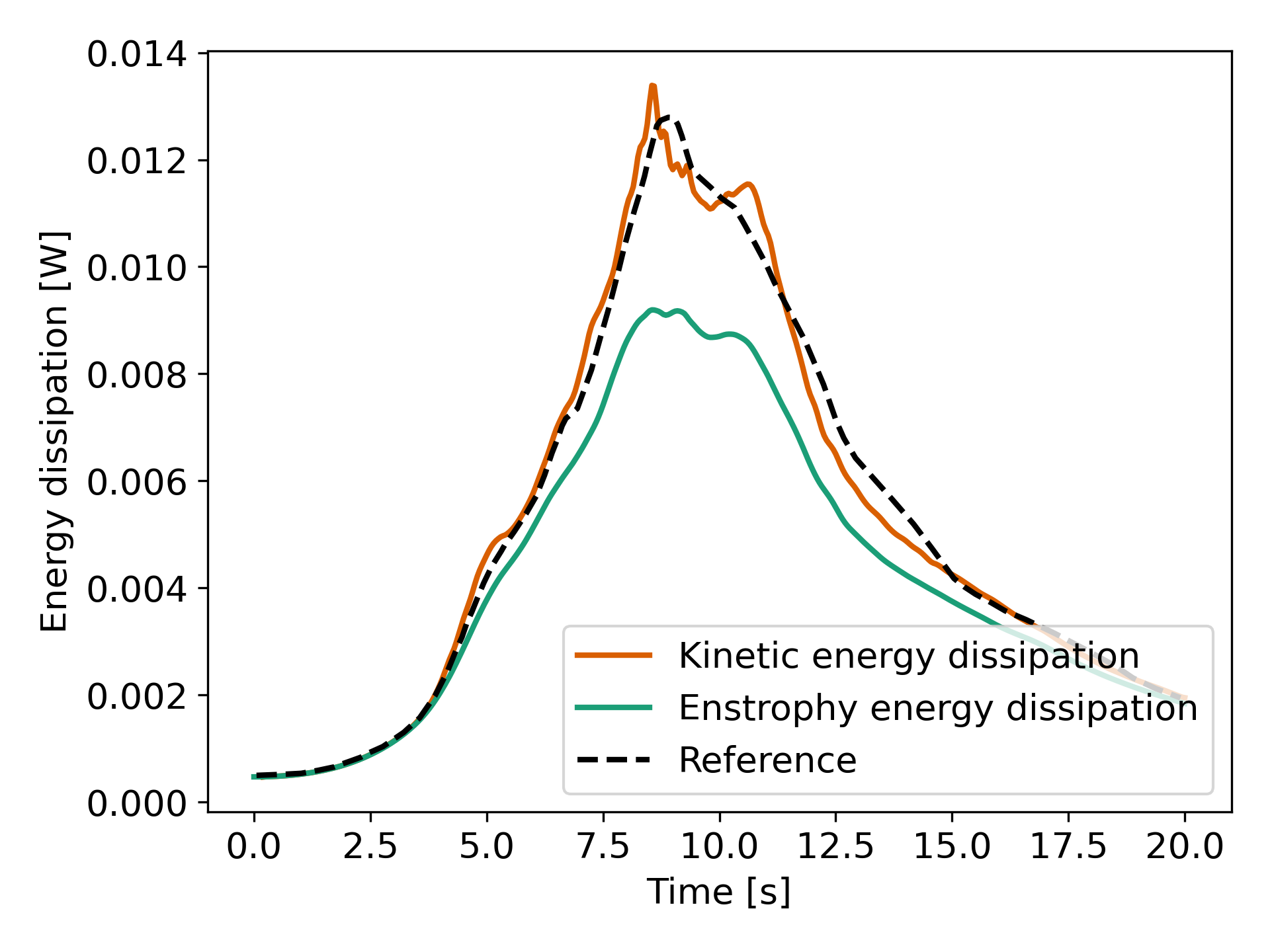
By refining the mesh once more (\(64^3\) Q3Q3) and decreasing the time step by a factor two (\(\Delta t=0.025\)), we recover the right kinetic energy decay, but we still observe significant numerical dissipation. These results are thus implicit LES where the SUPG/PSPG stabilization is acting as the subgrid scale model and mimics the kinetic energy decay that is not captured by the mesh.

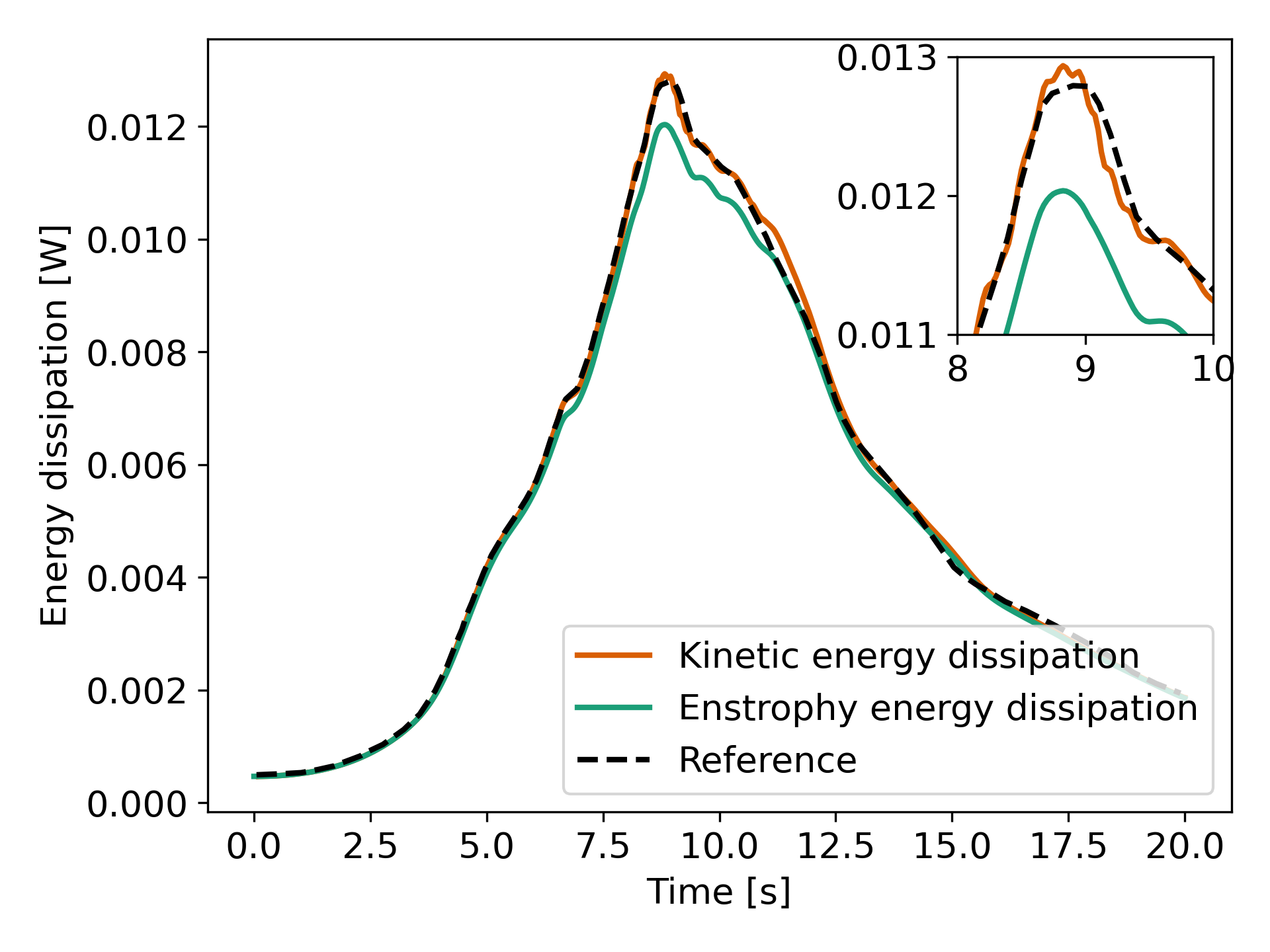
Increasing the refinement once more (\(128^3\) Q3Q3), allows us to obtain perfect agreement between the kinetic energy decay, the enstrophy and the reference results. These results constitute a Direct Numerical Simulation (DNS):

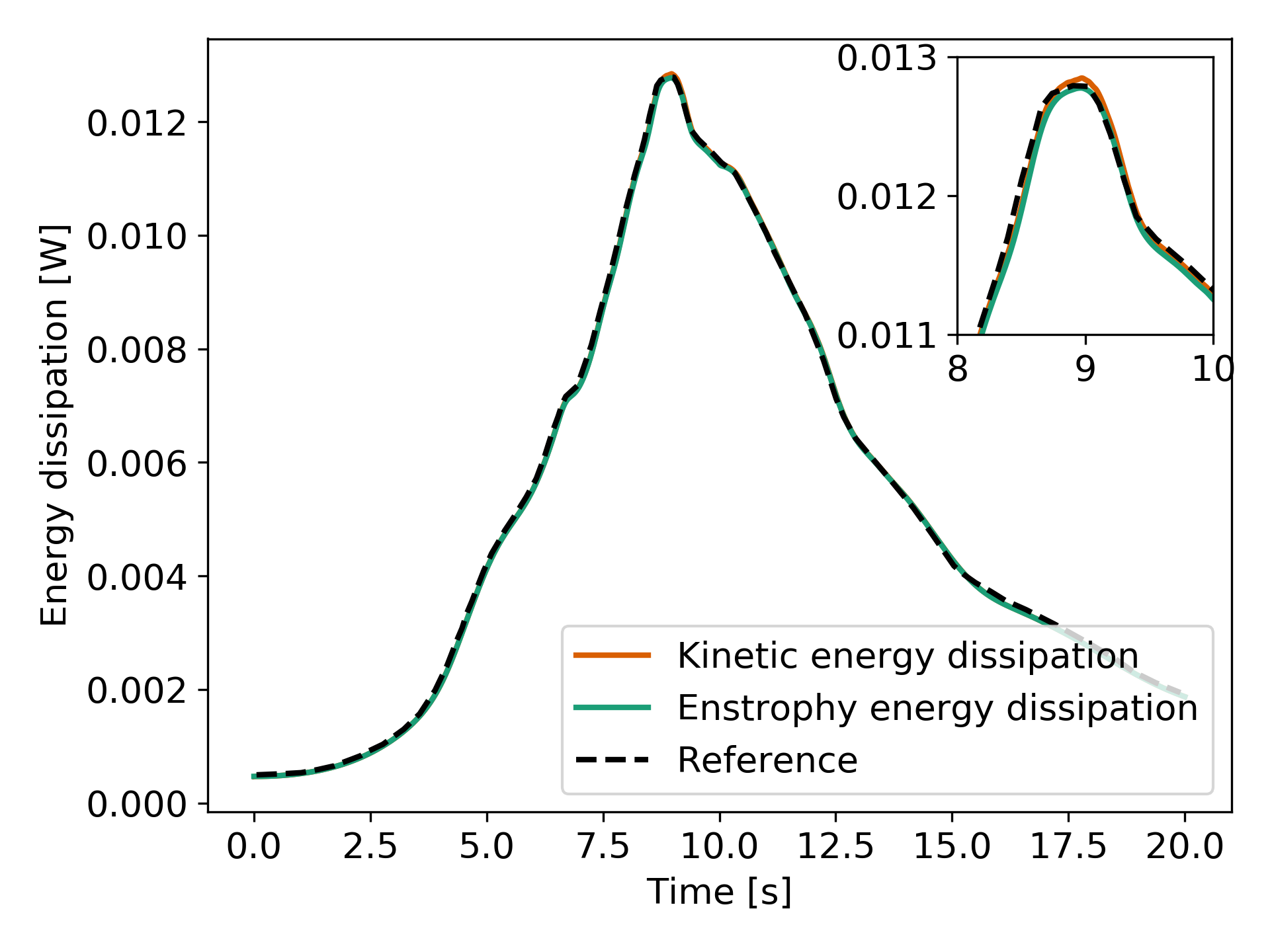
Possibilities for Extension

• This case is very interesting to postprocess. Try to postprocess this case using other quantities (vorticity, q-criterion) and use the results to generate interesting animations. Feel free to share them with us!

References

[1]

“Taylor–Green vortex,” Wikipedia. Dec. 01, 2023. Available: https://en.wikipedia.org/wiki/Taylor%E2%80%93Green_vortex.

[2]

Z. J. Wang et al., “High-order CFD methods: current status and perspective,” Int. J. Numer. Meth. Fluids, vol. 72, no. 8, pp. 811–845, 2013, doi: 10.1002/fld.3767.