Taylor-Couette Flow Using Nitsche Immersed Boundary#
This example revisits the same taylor-couette flow [1] problem in Taylor-Couette Flow, now using immersed boundaries to represent the inner cylinder. This example demonstrates some of the capabilities of Lethe to simulate the flow around complex geometries without meshing them explicitly with a conformal mesh, but instead by using the Nitsche immersed boundary method available within Lethe.
Features#
Solvers:
lethe-fluid-nitsche(with Q1-Q1, Q2-Q1 and Q2-Q2)
Note
We have not found that Q2-Q2 elements lead to better results when the flows are at a low Reynolds number.
Steady-state problem
Displays the use of an adaptive mesh refinement using Nitsche immersed boundaries
Displays the use of the analytical solution to calculate the mesh convergence
Displays the calculation of the torque induced by the fluid on a boundary
Files Used in This Example#
Both files mentioned below are located in the example’s folder (examples/incompressible-flow/2d-taylor-couette-nitsche).
Parameter file with uniform mesh refinement:
uniform-taylor-couette-nitsche.prmParameter file with adaptive mesh refinement:
adaptive-taylor-couette-nitsche.prm
Description of the Case#
Taylor-Couette flow is the name of a fluid flow in the gap between two long concentric cylinders with different rotational velocities. We simulate the same case as the regular Taylor-Couette flow where the inner cylinder rotates at a constant angular anti-clockwise velocity \(\omega\), while the outer cylinder is fixed. The following figure shows the geometry of this problem and the corresponding boundary conditions.

Parameter File#
We first establish the meshes used for the simulation. Using Nitsche immersed boundaries, two meshes are to be defined : the fluid mesh and the geometry mesh (i.e. the inner cylinder).
Mesh#
The mesh subsection specifies the computational grid:
subsection mesh
  set type               = dealii
  set grid type          = hyper_ball
  set grid arguments     = 0, 0 : 1 : true
  set initial refinement = 3
end
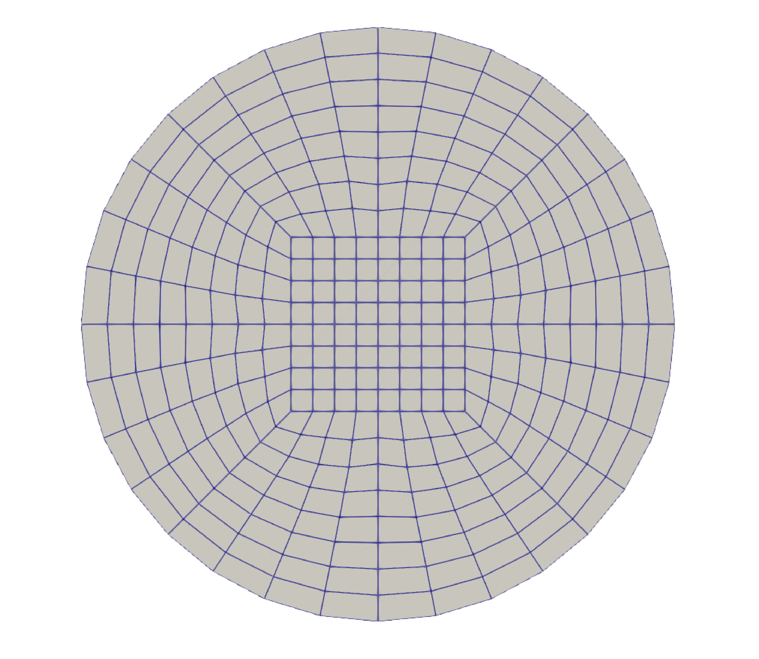
The type specifies the mesh format used. We use the hyper_shell mesh generated from the deal.II GridGenerator. This GridGenerator generates the mesh of the interstice between two concentric cylinders. The arguments of this grid type are the position of center of the cylinders (0, 0), the inner cylinder radius (0.25), the outer cylinder radius (1) and the number of subdivisions in the azimuthal direction (4). All arguments are separated by :. We set colorize=true and this sets the boundary ID of the inner cylinder to 0 and of the outer cylinder to 1
The last parameter specifies the initial refinement of the grid.
Note
Most deal.II grid generators contain a minimal number of cells. The 2D hyper_ball mesh is made of five cells, a square one in the middle and four ones surrounding it. Indicating an initial refinement=3 implies that the initial mesh is refined 3 times. In 2D, each cell is divided by 4 per refinement. Consequently, the final grid is made of 320 cells.
Nitsche Mesh#
The Nitsche subsection specifies the solid geometry embedded in the fluid domain. The Nitsche Immersed Boundary (IB) uses particles located at the
Gauss quadrature points of the immersed mesh to represent the immersed body. For a thorough explanation of this, we refer the reader to step-70 of deal.II.
subsection nitsche
  set verbosity        = verbose
  set number of solids = 1

  subsection nitsche solid 0
    set beta             = 10
    subsection mesh
      set type               = dealii
      set grid type          = hyper_ball
      set grid arguments     = 0, 0 : 0.25 : true
      set initial refinement = 6
    end
    subsection solid velocity
      set Function expression = -y ; x
    end
    set calculate torque on solid = true
  end
end
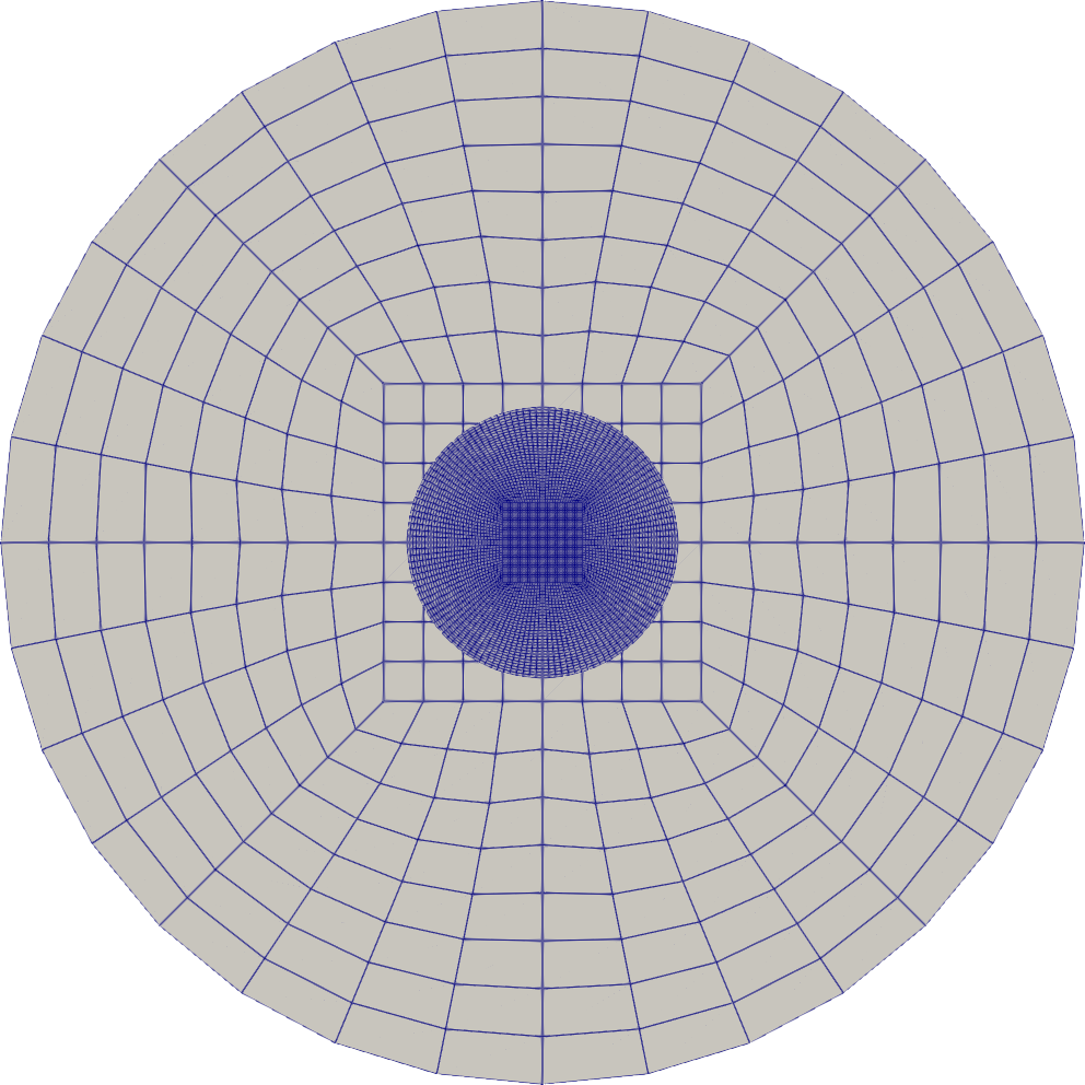
First, we set the number of solids to specify the amount of geometries that will be represented with Nitsche IB. For each Nitsche IB solid, we need to specify a beta coefficient, a mesh and a solid velocity. The beta coefficient is a parameter used to enforce the Nitsche IB. Its value is generally between 1 and 100 (10 being a reasonable value). The restriction automatically scales with the mesh size. In the case of the mesh, we note that in this problem, the Nitsche solid grid has the same dimension as the background grid. This is necessary for 2D simulations. Also, the Nitsche solid grid is well-refined to ensure that at approximately each fluid cell contains one particle of the immersed body. The solid velocity of the Nitsche IB is specified using the solid velocity subsection. By default, the motion of the particle is disabled. This means that even if the immersed particles have a non-zero velocity, they will not physically move in the fluid domain. In this case, this is useful because our problem has rotation symmetry and we will be seeking steady-state solutions. Finally, we enable the calculation of the torque on the Nitsche IB by setting calculate torque on solid = true.
The following figure illustrates the background mesh as well as the particles used to represent the IB on top of it:
Boundary Conditions#
The boundary conditions subsection becomes simple since the inner cylinder boundaries were specified in the previous section.
subsection boundary conditions
  set number = 1
  subsection bc 0
    set id   = 0
    set type = noslip
  end
end
First, the number of boundary conditions to be applied must be specified. For each boundary condition, the id of the boundary as well as its type must be specified. The outer cylinder (0) is static and, consequently, a noslip boundary condition is applied.
Physical Properties#
The analytical solution for the Taylor-Couette problem is only valid at low Reynolds number. We thus set the kinematic viscosity to 1.
subsection physical properties
  subsection fluid 0
    set kinematic viscosity = 1.0
  end
end
FEM Interpolation#
Note
In Example 2 we have used Q2 (quadratic) elements for velocity. In this problem, since we are using immersed boundary conditions, moving to higher degree polynomials would not enhance the order of convergence as the solid boundary is not represented with high accuracy with the Nitsche immersed boundary method.
subsection FEM
  set velocity degree = 1
  set pressure degree = 1
end
Analytical Solution#
Like in the first Taylor-Couette example, we add an analytical solution section to the parameter handler file. This analytical solution is more complex to define,
since the simulation domain encompasses the inside of the inner cylinder as well as the gap between the cylinders. Because of this, we only specify the analytical
solution for the velocity field and forego pressure. The analytical solution is only defined in the .prm file and we do not reproduce it here for the sake of brevity.
Forces#
The forces subsection controls the postprocessing of the torque and the forces acting on the boundaries of the domain.
subsection forces
  set verbosity             = verbose   # Output force and torques in log
  set calculate torque      = true      # Enable torque calculation
  set torque name           = torque    # Name prefix of torque files
  set calculation frequency = 1         # Frequency of the force calculation
  set output frequency      = 1         # Frequency of file update
end
By setting calculate torque = true, the calculation of the torque resulting from the fluid dynamics physics on every boundary of the domain is automatically calculated.
Setting verbosity=verbose will print out the value of the torque calculated for each mesh.
Simulation Control and Mesh Refinement#
As stated above, this problem can either be solved using a uniform mesh refinement or using an adaptive mesh refinement
Uniform Mesh Refinement#
The simulation control subsection controls the flow of the simulation. Two additional parameters are introduced in this example.
By setting number mesh adapt=4 we configure the simulation to solve the fluid dynamics on the mesh and on four(4) subsequently refined mesh.
This approach is very interesting, because the solution on the coarse mesh also serves as the initial guest for the solution on the finer mesh.
subsection simulation control
  set method            = steady
  set number mesh adapt = 4
  set output name       = taylor_couette_22
  set output frequency  = 1
  set output path       = ./
end
We then set the mesh adaptation type to uniform.
subsection mesh adaptation
  set type = uniform
end
Adaptive Mesh Refinement#
Since the Nitsche IB method introduces additional error on the surface of the immersed geometry, it is pertinent to investigate the results it can produce with adaptive mesh refinement. We now consider the following option:
subsection simulation control
  set method                  = steady
  set number mesh adapt       = 6
  set output name             = taylor_couette_22
  set output frequency        = 1
  set output path             = ./
end
The mesh can be dynamically adapted using Kelly error estimates on the velocity, pressure or variables arising from other physics.
subsection mesh adaptation
  set type                 = adaptive
  set error estimator      = kelly
  set variable             = velocity
  set fraction type        = number
  set max number elements  = 500000
  set max refinement level = 15
  set min refinement level = 0
  set frequency            = 1
  set fraction refinement  = 0.3
  set fraction coarsening  = 0.15
end
Rest of the Subsections#
The non-linear solver and linear solver subsections do not contain any new information in this example.
Running the Simulation#
Launching the simulation is as simple as specifying the executable name and the parameter file. Assuming that the lethe-fluid-nitsche executable is within your path, the simulation can be launched by typing:
or
Lethe will generate a number of files. The most important one bears the extension .pvd. It can be read by popular visualization programs such as Paraview.
Results and Discussion#
Uniform Mesh Refinement#
For the uniform mesh refinement problem, the evolution of the L2 error is as follows:
cells error_velocity  error_pressure
  320 2.6290e-02    - 1.5068e-02     -
 1280 1.2266e-02 1.10 1.9538e-02 -0.37
 5120 6.2622e-03 0.97 1.7759e-02  0.14
20480 3.2062e-03 0.97 1.7740e-02  0.00
81920 1.5688e-03 1.03 1.7626e-02  0.01
We discard the results for pressure since we have not specified an analytical solution. We note that as the number of cells increases, the error converges to zero at first order (error is divided by two when the mesh size decreases by a factor of two).
The torque on the inner cylinder is given in the torque_solid.00.dat file:
cells     T_x          T_y          T_z
  320 0.0000000000 0.0000000000 -0.6901522094
 1280 0.0000000000 0.0000000000 -0.7673814310
 5120 0.0000000000 0.0000000000 -0.8009318544
20480 0.0000000000 0.0000000000 -0.8186962282
81920 0.0000000000 0.0000000000 -0.8283917140
whereas the toque on the outer cylinder is given by the torque.00.dat file:
cells     T_x          T_y          T_z
  320 0.0000000000 0.0000000000 0.7223924685
 1280 0.0000000000 0.0000000000 0.7840745866
 5120 0.0000000000 0.0000000000 0.8093268556
20480 0.0000000000 0.0000000000 0.8229078025
81920 0.0000000000 0.0000000000 0.8305030116
We see that the sum of both torque converge towards zero as the mesh is refined, ensuring that Newton’s third law is respected. The torque on the inner cylinder should be -0.83776 and we note that the torque on both cylinder converges close to that value. Running the simulation with finer meshes lead to this results.
adaptive Mesh Refinement#
Using Paraview, the steady-state velocity profile can be visualized for the adaptive mesh refinement case:
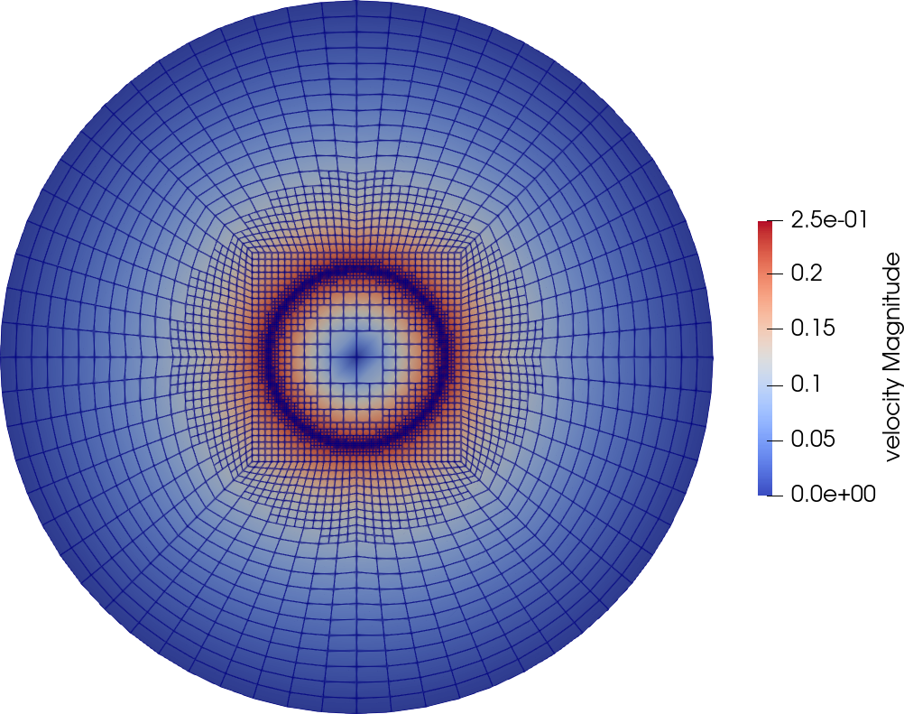
The end of the simulation log provides the following information about the convergence of the error:
cells error_velocity   error_pressure
  320 2.6280e-02    - 1.5068e-02     -
  620 1.2500e-02 1.07 1.9900e-02 -0.40
 1196 6.4573e-03 0.95 1.7950e-02  0.15
 2312 3.3532e-03 0.95 1.8708e-02 -0.06
 4580 1.5891e-03 1.08 1.7682e-02  0.08
 9056 8.4245e-04 0.92 1.7687e-02 -0.00
18284 4.3930e-04 0.94 1.8065e-02 -0.03
Correspondingly, the torque on the inner cylinder:
cells     T_x          T_y           T_z
  320 0.0000000000 0.0000000000 -0.6902135017
  620 0.0000000000 0.0000000000 -0.7681788397
 1196 0.0000000000 0.0000000000 -0.8020340261
 2312 0.0000000000 0.0000000000 -0.8196041387
 4580 0.0000000000 0.0000000000 -0.8289292869
 9056 0.0000000000 0.0000000000 -0.8332883003
18284 0.0000000000 0.0000000000 -0.8353647429
We see that even for a small number of cells (~18k), the error on the torque is less than 0.5%.
Possibilities for Extension#
Calculate formally the order of convergence for the torque \(T_z\).
It could be very interesting to investigate this flow in 3D at a higher Reynolds number to see the apparition of the Taylor-Couette instability.