Flow around a Cylinder

This example corresponds to a flow around a fixed cylinder. This is a classical problem studied in fluid mechanics. This example introduces several important features supported by Lethe.

Features

• Solver: lethe-fluid (with Q1-Q1)

• Steady-state problem

• Shows how to import a gmsh file

• Explains how to set a manifold

• Specifies an initial condition

• Displays the use of non-uniform mesh adaptation

Files Used in This Example

All files mentioned below are located in the example’s folder (examples/incompressible-flow/2d-flow-around-cylinder).

• Geometry file: cylinder-structured.geo

• Mesh file: cylinder-structured.msh

• Parameter file: cylinder.prm

Description of the Case

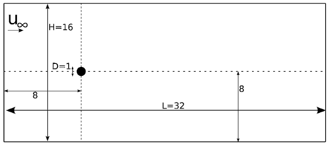
We simulate the flow around a fixed cylinder with a constant upstream fluid velocity. The following schematic describes the geometry with its relevant quantities (taken from the article by Blais et al. [1]):

Parameter File

Only the subsections of the parameter file that change significantly in comparison to Lid-Driven Cavity Flow and Taylor-Couette Flow examples are explained in this section.

Mesh

Lethe supports the use of imported mesh files:

subsection mesh
  set type      = gmsh
  set file name = cylinder-structured.msh
end

The type specifies the mesh format used, in this case we have gmsh which corresponds to a file generated by Gmsh. The set file name command specifies the path to the file. In this case, we assume that the parameter and mesh files are in the same folder. The .geo used to generate the gmsh mesh is provided.

Note

Assuming that the gmsh executable is within your $PATH variable, you may generate the .msh file from the example folder by typing:

gmsh -2 cylinder-structured.geo -o cylinder-structured.msh

Mesh Adaptation

This example uses a non-uniform mesh adaptation. The parameters used are specified in the mesh adaptation subsection:

subsection mesh adaptation
  set type                 = kelly
  set variable             = velocity
  set fraction type        = number
  set max number elements  = 70000
  set max refinement level = 6
  set min refinement level = 0
  set frequency            = 1
  set fraction refinement  = 0.3
  set fraction coarsening  = 0.1
end

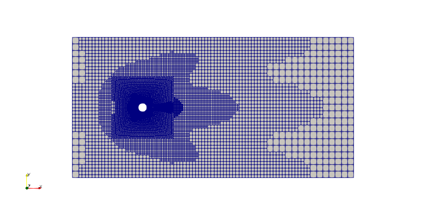
For steady-state simulations, one can enable a fixed number of mesh adaptations in the simulation control subsection. For this example, in the simulation control subsection (see Simulation Control), the following line is added: set number mesh adapt = 4. This means that the mesh will be adapted 4 times following the parameters specified in this subsection. In this case the type is set to kelly which corresponds to the Kelly Error Estimator strategy as implemented in deal.II, and calculated with respect to the velocity variable. For more details on the different parameters and options refer to the Parameters Guide.

The result of this mesh adaptation can be clearly seen if we compare the initial mesh:

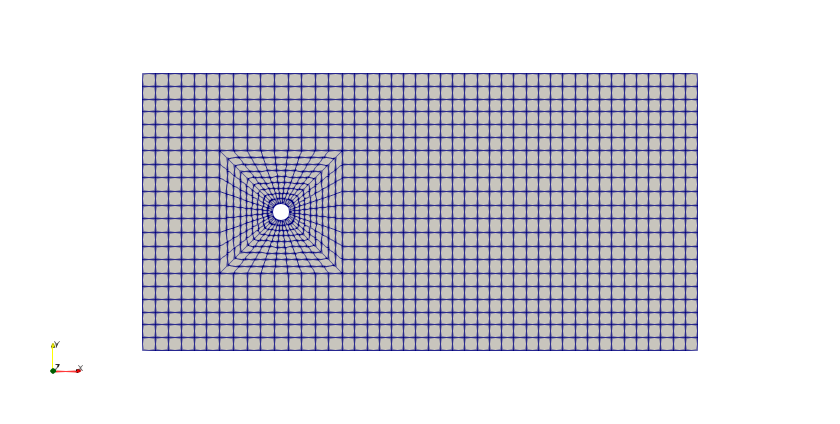
and the final mesh after being adapted 4 times:

Manifolds

All the deal.II meshes supported by Lethe that correspond to the GridGenerator class, attach by default manifolds to meshes when needed. However, if another type of mesh is used in Lethe, it is possible to attach manifolds adding a section to the parameter file that looks as follows:

subsection manifolds
  set number = 1
  subsection manifold 0
    set id   = 0
    set type = spherical
    set point coordinates = 8, 8
  end
end

First the number of manifolds is specified by the set number command. Then a subsection for each of the manifolds is created starting with the manifold 0. The boundary id is in this case set to 0 as we want to set a spherical manifold and this is the corresponding id in this example. Then the type of the manifold is specified. For more information on the types of manifolds supported in Lethe, we refer to the Manifolds section.

Note

For more information about manifolds and the way they can be leveraged for simulations, we invite you to read the documentation page of deal.II: Manifold description for triangulations.

Initial Conditions

Despite this problem being a steady-state problem, one known strategy to improve convergence is to set a coherent initial condition. In Lethe, this can be achieved by the initial conditions subsection:

subsection initial conditions
  set type = nodal
  subsection uvwp
    set Function expression = 1; 0; 0
  end
end

In this case we use the nodal initial condition and the subsection uvwp allows the description of a velocity-pressure vector-valued function. It can be seen that the individual components of the function are separated by semicolons in the set Function expression. In this case, the velocity in the x-direction is set to 1, the velocity in the y-direction is set to 0, and the pressure is set to 0. If the problem was in three dimensions, four values should be specified, velocity in x, y and z directions and the pressure.

Boundary Conditions

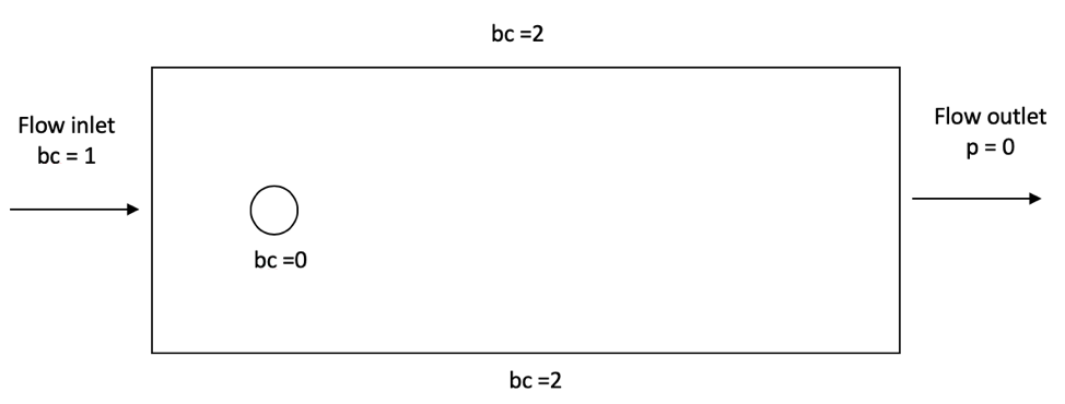
In this section, we specify the boundary conditions taking into account the IDs presented in the following schematic:

subsection boundary conditions
  set number = 4
  subsection bc 0
    set type = noslip
  end
  subsection bc 1
    set type = function
    subsection u
      set Function expression = 1
    end
    subsection v
      set Function expression = 0
    end
    subsection w
      set Function expression = 0
    end
  end
  subsection bc 2
    set type = slip
  end
  subsection bc 3
    set type = outlet
  end
end

• bc 0 identifies the cylinder where we apply noslip boundary conditions on its walls. This leads to a velocity \(\mathbf{u} = \mathbf{0}\) for the fluid directly in contact with the walls of the cylinder.

• bc 1 determines the flow of the fluid from the left wall. As mentioned before, the fluid is moving in the x-direction and therefore its boundary condition is defined with a function having a u velocity equals to 1. The rest of the velocity components are set to 0.

• bc 2 is applied at the top and bottom walls. This condition allows the simulation to be performed in a finite sized domain. In real life, the cylinder would be placed in a relatively infinite domain. Using slip condition, we assume that the fluid cannot go out in the normal direction, but that it can still flow from left to right without friction. Thus, the walls have no effect on the flow of the fluid.

• bc 3 is applied at the right extremity of the domain to impose an outlet boundary condition. In essence, this corresponds to a natural boundary condition where the pressure \(p\) becomes close to 0 due to the imposed \(\int_{\Gamma}(-p\mathcal{I} + \mathbf{\tau}) \cdot \mathbf{n}=0\). For more details, refer to Boundary Conditions - CFD section.

Forces

To calculate forces acting on the boundary conditions, for example, the forces acting on the cylinder, we can use the forces subsection:

subsection forces
  set verbosity             = verbose
  set calculate force       = true
  set calculate torque      = false
  set force name            = force
  set output precision      = 10
  set calculation frequency = 1
  set output frequency      = 1
end

To print the values of the forces in the terminal we set verbosity to verbose. The calculation of the forces in all boundaries is set by the set calculate force = true line. A .dat file is created with the corresponding data. Therefore, one can specify the prefix of the file by the force name parameter, the number of significant digits for the force values by the output precision and the frequency of calculation and output which are set to 1.

Running the Simulation

The mesh must be generated before the simulation is launched. A gmsh file is provided in this example and it can be used to generate the mesh of the domain:

gmsh -2 cylinder-structured.geo

Launching the simulation is as simple as specifying the executable name and the parameter file. Assuming that the lethe-fluid executable is within your path, the simulation can be launched by typing:

lethe-fluid cylinder.prm

Lethe will generate a number of files. The most important one bears the extension .pvd. It can be read by visualization programs such as Paraview.

Results and Discussion

Using Paraview the following steady-state velocity and pressure profiles can be visualized:

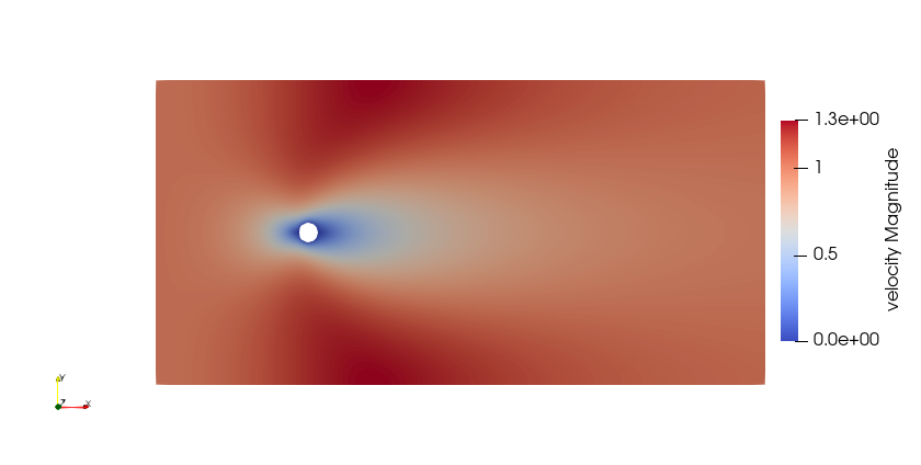
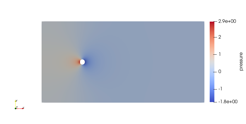
From the velocity distribution, we notice how the velocity of the fluid is 0 at the boundaries of the cylinder and how it increases gradually if we move further away from it. In the case of the pressure, the difference between the inlet and outlet is visible and we can see how the pressure is near to 0 close to the outlet.

In addition to these profiles, we also obtain the values of the forces acting on the cylinder. These values can be found on the forces.00.dat file produced by the simulation and correspond to the forces acting on the bc 0 (cylinder boundary). The force is decomposed in its two components which are the viscous force (f_v) due to shear stresses on the boundary, and a pressure force (f_p) due to the body shape.

cells     f_x           f_y          f_z          f_xv         f_yv          f_zv         f_xp         f_yp          f_zp
 1512 6.6313161094  0.0000000557 0.0000000000 3.0711960956  0.0000000291 0.0000000000 3.5601200138  0.0000000266 0.0000000000
 2874 6.9728845035 -0.0000000813 0.0000000000 3.2624415260 -0.0000000337 0.0000000000 3.7104429775 -0.0000000477 0.0000000000
 5460 7.0836039086  0.0002060398 0.0000000000 3.3909108964  0.0001138765 0.0000000000 3.6926930122  0.0000921633 0.0000000000
10374 7.0934695138 -0.0000295671 0.0000000000 3.4455331107 -0.0000147141 0.0000000000 3.6479364031 -0.0000148530 0.0000000000
19521 7.1110693811  0.0000390078 0.0000000000 3.4735982034  0.0000254535 0.0000000000 3.6374711776  0.0000135542 0.0000000000

The force in the x direction is the parallel or drag force, while the force in the y direction is the perpendicular or lift force. The drag and lift coefficients can be calculated as follows:

\[C_D = \frac{2 f_x}{\rho U_\infty^2 D}, C_L = \frac{2 f_y}{\rho U_\infty^2 D}\]

where \(U_\infty\) is the upstream velocity and \(D\) is the diameter of the cylinder. Considering the small values of the lift force, we calculate only the drag coefficients:

Cells   C_D
1512    13.26
2874    13.94
5460    14.16
10374   14.18
19521   14.22

We can see that the simulation is mesh convergent, as the last three values of the force in the x-direction and therefore the drag coefficient differ in less than 1%. An experimental value of the drag coefficient as a function of the Reynolds number is available in the Drag Coefficient Calculator , and for a Reynolds number of 1, it corresponds to a value of \(C_D = 11.9\). The value calculated by Lethe differs from the theoretical value because of the slip boundary condition at the top and bottom walls, along with the short distance to them from the surface of the cylinder. To obtain a more accurate drag coefficient, the geometry should be enlarged.

Possibilities for Extension

• Play with the size of geometry to observe the effect on the calculation of the drag forces.

• Increase the Reynolds number and perform an unsteady simulation to observe the famous von Kármán vortex street pattern.

• It would be interesting to try the same example in 3D and observe what happens with the drag and lift forces.

Reference

[1]

B. Blais, M. Lassaigne, C. Goniva, L. Fradette, and F. Bertrand, “A semi-implicit immersed boundary method and its application to viscous mixing,” Comput. Chem. Eng., vol. 85, pp. 136–146, Feb. 2016, doi: 10.1016/j.compchemeng.2015.10.019.