3D Static Mixer Using RBF Sharp Immersed Boundary

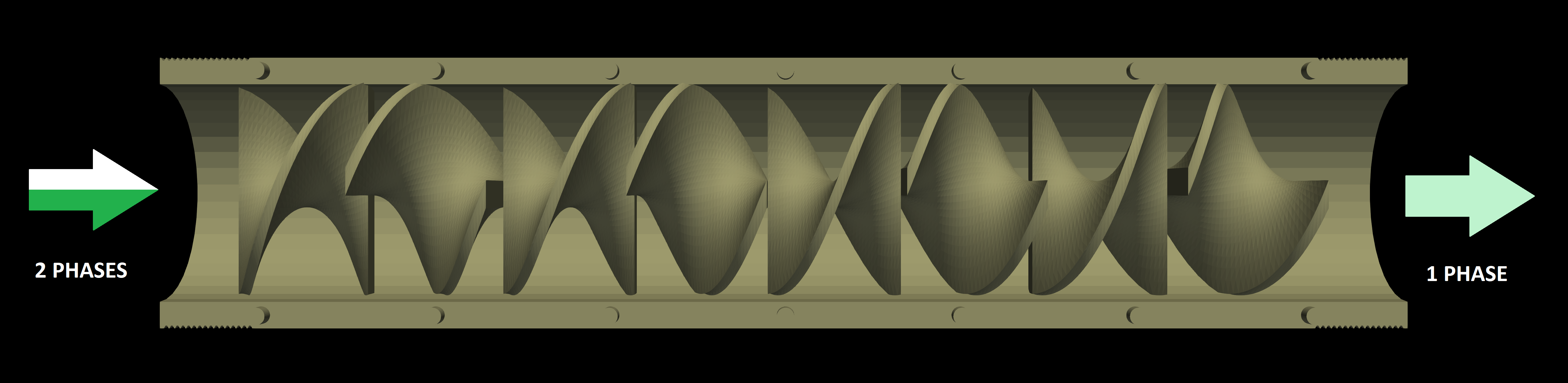
The usage of static mixers is common for the blending of multi-component products in polymerization, as well as water treatment and chemical processing. They involve no moving part, but obtain mixing effects by converting the pressure gradient to radial mixing and flow division as the flow progresses through obstacles. Their advantages include low maintenance, no external energy input, continuous operation, compact design (pipe insertion), and easy installation.

As opposed to stirred tanks, it is not possible to modulate rotation speed or change the impeller. Hence, the design of these systems must be approached with precision due to these limitations. Factors such as the desired level of mixing and the properties of the fluids involved must be carefully considered.

Features

• Solvers: lethe-fluid-sharp

• Transient problem

• Complex static solid defined by a surface grid (STL) and modeled with the Radial Basis Function (RBF) sharp immersed boundary method

Files Used in This Example

All files mentioned below are located in the example’s folder (/examples/sharp-immersed-boundary/3d-rbf-static-mixer/).

RBF preparation files:

• Parameter file: rbf_generation/RBF.param;

• Surface grid file: rbf_generation/helix.stl. This surface grid was taken from Thingiverse [1] under CC BY 4.0.

Lethe’s fluid simulation files:

• Composite geometry file: lethe_sharp_simulation/mixer_long.composite;

• Parameter file: lethe_sharp_simulation/flow_in_long_mixer.prm;

• RBF geometry file: lethe_sharp_simulation/RBF_helix.output. The extension is .output because it was named from a bitpit perspective.

Description of the Case

In this example, we showcase the RBF type of objects used in Lethe’s resolved immersed-boundary Navier-Stokes solver.

Preparation of the Solid

Generation of the RBF file from the STL

bitpit is an open-source modular library for scientific computing. The current section presents an example using its RBF capabilities to train RBF-networks that approximate the geometry from surface grid objects (.stl).

Tip

In order to install bitpit, you need to have the github version of PETSc, which itself requires BLAS/LAPACK and LibXML2. In order, BLAS/LAPACK and LibXML2 must be installed, then PETSc, then bitpit.

For the dependencies installation, you can use:

sudo apt-get install libblas-dev liblapack-dev liblapacke-dev libxml2-dev

For the PETSc installation, you must first create a directory for the installation, then clone the project and configure it. Here are a few lines to help set it up:

cd /home/
mkdir software
cd software
git clone -b release https://gitlab.com/petsc/petsc.git petsc
cd petsc
git pull
./configure
make all check

For the bitpit installation, you must first create a directory for the installation, then clone the project and build it (ideally in a separate directory). The dependencies’ paths must be specified. Here are a few lines to help compile bitpit with 6 processes:

cd /home/
mkdir software
cd software
mkdir bitpit
cd bitpit
git clone https://github.com/optimad/bitpit
mkdir build
cd build
cmake ../bitpit/ -DBITPIT_BUILD_EXAMPLES=ON -DPETSC_DIR=/path/to/petsc/installation/ -DPETSC_ARCH=arch-linux-c-debug
make -j6

After compiling the library, we can use an executable /examples/RBF_example_00001, along with a parameter file and the helix.stl in the rbf_generation directory.

The parameter file (RBF.param) contains:

nb_subdivision nb_adaptions radius_ratio base_function mesh_range
16             4            3            1             0.1

1. The number of subdivisions in each of the three spatial dimensions: 16;

2. The number of adaption cycles. Using 4 adaptation cycles over a initial number of 16 subdivisions results in a level of detail equivalent to a number of 256 subdivisions;

3. The radius ratio means that each node sees up to 3 neighbors in each direction, which results in a smooth approximation.

4. The base function of 1 means that the basis function is of Wendland type. This is the best function to represent geometries from our experience.

5. The mesh range of 0.1 means that there is at least 10% of margin on each side of the object, so the collection of RBF nodes are encompassing the whole object.

Assuming that the RBF_example_00001 executable is within your $PATH or copied to /rbf_generation/ directory, we can launch the RBF generation from /rbf_generation/ using the command line:

RBF_example_00001 ./ helix RBF.param

After about 40 minutes this executable will output RBF_helix.output, which is the encoding of the shape, and RBF_helix.vtu, which can be used to see the resulting approximation.

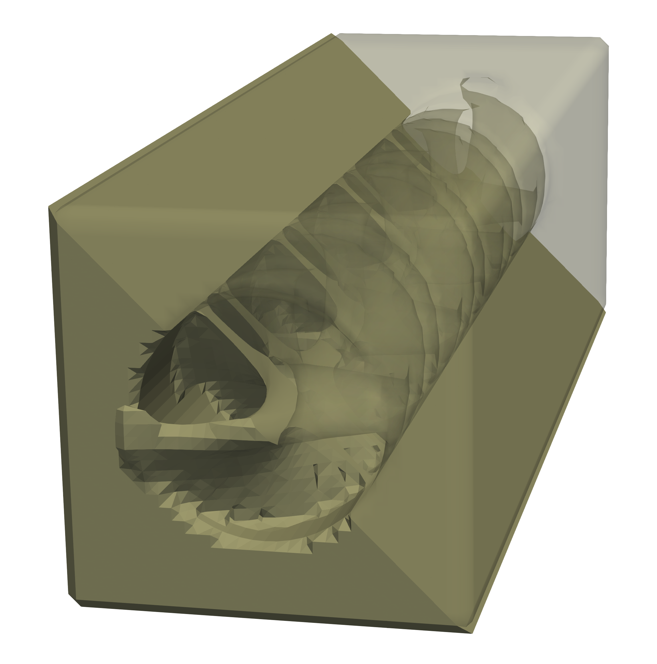
Creation of the Composite Shape File

The complete geometry through which the fluid flows contains the helix static mixer as well as the casing around it. We use composite shapes to build the complex geometry; this type of shape is introduced in this example: Simple Plane Model From Composite. The main particularities of the current composite shape are:

1. The translation parameter for the rbf shape is -76.201:-20.0098:+15.6051. It is selected to ensure that the center of the static mixer is located at the origin. The coordinates are taken from rbf_generation/bitpit.log.

2. The hyper rectangle is long enough to cover the length of the helix, and just large enough to fit in the background grid.

3. The cylinder hole is set to have a very high length to ensure that the difference operation applies properly over the whole domain.

4. Operation 15 forms the casing, and operation 16 joins the casing and the helix. The final operation is the one considered as definitive.

shapes
0; rbf             ; RBF_helix.output;   -76.201:-20.0098:+15.6051;    0:+1.57079632679:0
1; hyper rectangle ;         75:25:25;                       0:0:0;                 0:0:0
2; cylinder        ;         15:10000;                       0:0:0;    0:+1.57079632679:0
operations
15; difference     ; 2:1
16; union          ; 0:15

Parameter File

Simulation Control

Although we are interested in the steady-state solution of the flow, we use bdf1 time integration. The required time to reach steady state in our case is low, but solving it with a small value of the time step enables the non-linear solver to converge as complex flow patterns are difficult to capture otherwise.

subsection simulation control
  set method      = bdf1
  set time end    = 40e-4
  set time step   = 1e-4
  set output path = ./output/
  set output name = output
end

Physical Properties

We assume that the fluid is water, and that the length of the static mixer is in the order of \(150 \, \text{cm}\). Hence, the length units are centimeters and the time units are seconds. The kinematic viscosity of water is \(0.01 \, \text{cm²}/\text{s}\).

subsection physical properties
  subsection fluid 0
    set kinematic viscosity = 0.01
  end
end

Mesh and Mesh Adaptation

The mesh is a simple hyper rectangle, large enough to encompass the mixer with its casing and long enough to establish the flow profile upstream and downstream.

subsection mesh
  set type      = dealii
  set grid type = subdivided_hyper_rectangle

  # Grid to use when solving the flow in the long version of the mixer
  set grid arguments = 6,1,1: -150,-25,-25: 150,25,25: true

  set initial refinement = 3
end

Mesh adaptation type is set to kelly, to allow adaptive refinement at the solid surface. This is necessary for simulations of this type because of the prohibitive mesh size required when only uniform refinement is used. Setting max refinement level = 5 allows for two levels of adaptive refinement from the uniform initial refinement = 3 defined in the mesh section. The frequency = 0 ensures that no refinement occurs between time steps, as it is not necessary here. The initial refinement steps = 0 to highlight that no initial refinement is requested here; the initial refinements are requested from subsection particles because they are base on the solid geometry.

subsection mesh adaptation
  set type                     = kelly
  set fraction type            = number
  set max number elements      = 2000000
  set max refinement level     = 5
  set min refinement level     = 0
  set frequency                = 0
  set initial refinement steps = 0
end

Definition of the Shape

This section defines each parameter for the particles and has certain requirements:

subsection particles
  set assemble Navier-Stokes inside particles = false
  set number of particles                     = 1

  subsection extrapolation function
    set length ratio  = 4
    set stencil order = 1
  end

  subsection local mesh refinement
    set initial refinement                = 4
    set refine mesh inside radius factor  = 1
    set refine mesh outside radius factor = 1
    set refinement zone extrapolation     = false
  end

  subsection particle info 0
    set type            = composite
    set shape arguments = mixer_long.composite
  end
end

1. In subsection extrapolation function, length ratio defines the length used to apply the immersed boundaries through interpolation. We choose 4 as a compromise between a low value, which is better for the linear solver, and a high value, which is better for mass preservation. The latter can also be increased using a finer grid.

2. In subsection local mesh refinement, refine mesh inside radius factor and refine mesh outside radius factor are both set to 1, which activates minimal crown refinement mode.

3. In subsection particle info 0, type = composite and shape arguments = mixer_long.composite define the shape itself. This requires that the RBF_helix.output is located in the same directory as the parameter file.

Boundary Conditions

A condition is assigned to each boundary:

1. The inlet is set to a Dirichlet boundary condition with unit velocity in the x direction.

2. The outlet is defined as such, and is the weakly imposed condition required when using lethe-fluid-sharp.

3. The remaining boundaries are set as noslip to emulate the flow in a channel.

subsection boundary conditions
  set number = 6
  subsection bc 0
    set id   = 0
    set type = function
    subsection u
      set Function expression = 1
    end
  end
  subsection bc 1
    set id   = 1
    set type = outlet
  end
  subsection bc 2
    set id   = 2
    set type = noslip
  end
  subsection bc 3
    set id   = 3
    set type = noslip
  end
  subsection bc 4
    set id   = 4
    set type = noslip
  end
  subsection bc 5
    set id   = 5
    set type = noslip
  end
end

Post-Processing

Pressure drop and flow rate post-processing are enabled to track when steady state is reached and to ensure that mass is preserved. Too high variations between inlet and outlet flow rates are linked to increased error on the pressure drop predictions.

subsection post-processing
  set verbosity               = verbose
  set calculate pressure drop = true
  set calculate flow rate     = true
  set inlet boundary id       = 0
  set outlet boundary id      = 1
end

Running the Simulation

The simulation can be launched on multiple cores using mpirun and the lethe-fluid-sharp executable. Using 6 CPU cores (for an approximate runtime of 50 minutes), the simulation can be launched with:

mpirun -np 6 lethe-fluid-sharp flow_in_long_mixer.prm

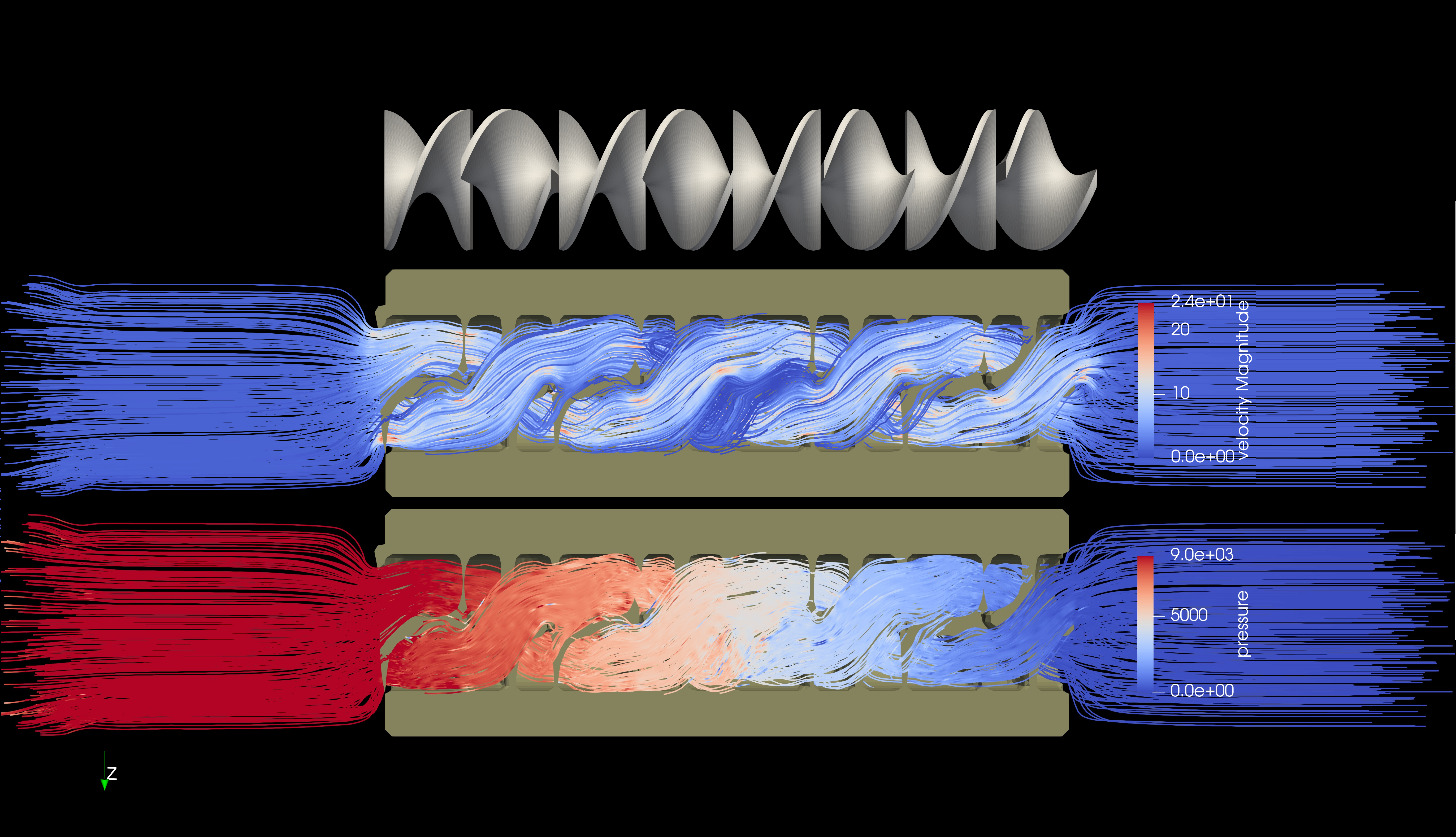
Results

After the simulation has run, streamlines can be used to visualize the pressure and velocity fields through the static mixer, as well as show the mixing effects that can be obtained.

The mass conservation and pressure drop can both be monitored by plotting their values in time, extracted from /output/flow_rate.dat and /output/pressure_drop.dat. The Python script postprocess_flow_and_pressure.py generates the following plot:

  python3 postprocess_flow_and_pressure.py

As the plot shows, the mass conservation is constant after only a few time steps; it depends mostly on the length ratio, residual and grid refinement. The pressure drop, on the other hand, decreases steadily. We stopped the simulation after 40 time steps because the decrease is then low enough, but increasing the total duration would be interesting to get a better idea of the steady-state pressure drop.

Reference

[1]

“Group 9., Helix Static Mixer,” Thingiverse Available: https://www.thingiverse.com/thing:3915237