Cylindrical Packed Bed

It is strongly recommended to visit DEM parameters and CFD-DEM parameters for more detailed information on the concepts and physical meaning of the parameters ind DEM and CFD-DEM.

Features

• Solvers: lethe-particles and lethe-fluid-vans

• Three-dimensional problem

• Uses the VANS solver without the coupling with DEM

• Displays the selection of models and physical properties

Files Used in This Example

Both files mentioned below are located in the example’s folder (examples/unresolved-cfd-dem/cylindrical-packed-bed).

• Parameter file for particle generation and packing: packing-particles.prm

• Parameter file for CFD-DEM simulation of the packed bed: flow-in-bed.prm

Description of the Case

This example simulates air flow through a packing of particles. First, we use lethe-particles to fill the bed with particles. We enable check-pointing in order to write the DEM checkpoint files which will be used as the starting point of the CFD-DEM simulation. Then, we use the lethe-fluid-vans solver within Lethe to simulate air flow through the packed bed.

DEM Parameter File

All parameter subsections are described in the parameter section of the documentation. To set-up the cylindrical packed bed case, we first fill the bed with particles. We introduce the different sections of the parameter file (packing-particles.prm) needed to run this simulation.

Mesh

In this example, we are simulating a cylindrical packed bed that has a half length of 0.1 m, and a radius of 0.01 m. We use the GridGenerator::subdivided_cylinder function of Deal.II in order to generate the mesh. The cylinder is divided 16 times in the x direction. The following portion of the DEM parameter file shows the function called. The mesh subsection specifies the computational grid:

subsection mesh
  set type               = dealii
  set grid type          = subdivided_cylinder
  set grid arguments     = 16:0.01:0.1
  set initial refinement = 1
end

Simulation Control

Another subsection, which is generally the one we put at the top of the parameter files, is the simulation control . time step, end time, log and output frequency are defined here. Additionally, users can specify the output folder for the simulation results in this subsection. The log frequency parameter controls the frequency at which the iteration number is printed on the terminal. If log frequency = 1000 the iteration number will be printed out every 1000 iterations. This is an easy way to monitor the progress of the simulation. A simulation time of 0.6 s was chosen with a time step of 1e-5 s. It it important to choose a long enough time as to allow all particles to come to rest. We store the output files generated in the folder output_dem:

subsection simulation control
  set time step        = 0.00001
  set time end         = 0.6
  set log frequency    = 1000
  set output frequency = 1000
  set output path      = ./output_dem/
end

Warning

If an output path is chosen, you need to create the folder before launching the simulation. Otherwise, an error message will appear and the simulation will fail to launch.

Restart

The volume-averaged Navier-Stokes (VANS) solver requires reading several DEM files. For this, we have to write the DEM simulation information. This is done by enabling the check-pointing option in the restart subsection. We give the written files a prefix lethe-particles set in the set filename option.

subsection restart
  set checkpoint = true
  set frequency  = 10000
  set filename   = dem
end

Model Parameters

The section on model parameters is explained in the DEM examples. We show the chosen parameters for this section:

subsection model parameters
  set contact detection method               = dynamic
  set contact detection frequency            = 10
  set neighborhood threshold                 = 1.3
  set particle particle contact force method = hertz_mindlin_limit_overlap
  set particle wall contact force method     = nonlinear
  set integration method                     = velocity_verlet
end

Lagrangian Physical Properties

The physical properties section of the particles allows us to determine the different parameters related to the particle such as its density, diameter, and the different coefficients that dictate the collision behaviour of the particles. Also, in this section we define the total number of particles for the simulation. The gravitational acceleration as well as the physical properties of particles and walls are specified in the lagrangian physical properties subsection. These properties include as well the Young’s modulus, Poisson’s ratio, restitution coefficient, friction and rolling friction coefficients.

subsection lagrangian physical properties
  set g                        = -9.8, 0.0, 0.0
  set number of particle types = 1
  subsection particle type 0
    set size distribution type            = uniform
    set diameter                          = 0.001
    set number                            = 10000
    set density particles                 = 2500
    set young modulus particles           = 1e6
    set poisson ratio particles           = 0.3
    set restitution coefficient particles = 0.2
    set friction coefficient particles    = 0.1
    set rolling friction particles        = 0.2
  end
  set young modulus wall           = 1e6
  set poisson ratio wall           = 0.3
  set restitution coefficient wall = 0.2
  set friction coefficient wall    = 0.1
  set rolling friction wall        = 0.3
end

Insertion Info

The insertion info subsection manages the insertion of particles. It allows us to control the insertion of particles at each time step. This section is already explained in the DEM examples. However, further information regarding the information box will be given. The volume of insertion box should be large enough to fit all particles. Also, its bounds should be located within the mesh generated in the Mesh subsection.

subsection insertion info
  set insertion method                               = volume
  set inserted number of particles at each time step = 500
  set insertion frequency                            = 1000
  set insertion box points coordinates               = 0, -0.01, 0 : 0.1, 0.01, 0.01
  set insertion distance threshold                   = 2.2
  set insertion maximum offset                       = 0.5
  set insertion prn seed                             = 19
end

Floating Walls

We need to pack the particles in the middle of the cylinder. Therefore, we create a stopper (floating wall) somewhere below the center of the cylinder. We chose the point with an x-coordinate of -0.01 to create the wall. We then define a normal to the wall at this point. We make sure that the end time of the floating wall is bigger than the simulation time to ensure that the particles remain suspended. This is shown in:

subsection floating walls
  set number of floating walls = 1
  subsection wall 0
    subsection point on wall
      set x = -0.01
      set y = 0
      set z = 0
    end
    subsection normal vector
      set nx = 1
      set ny = 0
      set nz = 0
    end
    set start time = 0
    set end time   = 2
  end
end

Running the DEM Simulation

Launching the simulation is as simple as specifying the executable name and the parameter file. Assuming that the lethe-particles executable is within your path, the simulation can be launched on a single processor by typing:

lethe-particles packing-particles.prm

or in parallel (where 8 represents the number of processors)

mpirun -np 8 lethe-particles packing-particles.prm

Lethe will generate a number of files. The most important one bears the extension .pvd. It can be read by popular visualization programs such as Paraview.

Note

The .vtu files generated by Lethe are compressed archives. Consequently, they cannot be postprocessed directly. Although they can be easily post-processed using Paraview, it is sometimes necessary to be able to work with the raw data. The python library PyVista allows us to do this.

Results DEM

Packed particles at the end of simulation:

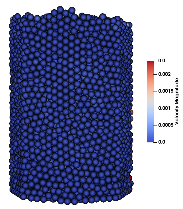
After the particles have been packed inside the cylindrical bed, it is now possible to simulate fluid flow through the packing.

VANS Parameter File

The CFD simulation is to be carried out using the packed bed simulated in the previous step. We will discuss the different parameter file sections. The mesh section is identical to that of the DEM so it will not be shown here.

Simulation Control

The simulation is run in steady state. The simulation control section is shown:

subsection simulation control
  set method            = bdf1
  set output name       = result
  set output path       = ./output/
end

Physical Properties

The physical properties subsection allows us to determine the density and viscosity of the fluid. We choose a density of 1 and viscosity of 0.00001 as to simulate the flow of air.

subsection physical properties
  subsection fluid 0
    set kinematic viscosity = 0.00001
    set density             = 1
  end
end

Initial Conditions

For the initial conditions, we choose zero initial conditions for the velocity.

subsection initial conditions
  set type = nodal
  subsection uvwp
    set Function expression = 0; 0; 0; 0
  end
end

Boundary Conditions

For the boundary conditions, we choose a slip boundary condition on the walls of the cylinder (ID = 0) and an inlet velocity of 0.2 m/s at the lower face of the cylinder (ID = 1).

subsection boundary conditions
  set number = 2
  subsection bc 0
    set id   = 0
    set type = slip
  end
  subsection bc 1
    set id   = 1
    set type = function
    subsection u
      set Function expression = 0.2
    end
    subsection v
      set Function expression = 0
    end
    subsection w
      set Function expression = 0
    end
  end
end

The additional sections that define the VANS solver are the void fraction subsection and the CFD-DEM subsection. These subsections are described in detail in the CFD-DEM parameters .

Void Fraction

Since we are calculating the void fraction using the packed bed of the DEM simulation, we set the mode to dem. For this, we need to read the dem files which we already wrote using check-pointing. We therefore set the read dem to true and specify the prefix of the dem files to be read. In order to ensure that our void fraction projection is bounded, we choose an upper bound limit of 1. We decide not to lower bound the void fraction and thus attributed a value of 0 to the L2 lower bound parameter. We now choose a smoothing factor for the void fraction as to reduce discontinuity which can lead to oscillations in the velocity. The factor we choose is around the square of twice the particle’s diameter.

subsection void fraction
  set mode                = pcm
  set read dem            = true
  set dem file name       = dem
  set l2 smoothing factor = 0.000005
end

CFD-DEM

We also enable grad_div stabilisation in order to improve local mass conservation.

Note

For certain simulations, this parameter should be disabled to improve stability of the solver.

subsection cfd-dem
  set grad div                      = true
  set drag force                    = true
  set buoyancy force                = true
  set shear force                   = false
  set pressure force                = false
  set drag model                    = rong
  set post processing               = true
  set vans model                    = modelB
end

We determine the drag model to be used for the calculation of particle-fluid forces. Currently, Difelice, Rong and Dallavalle models are supported. Other optional forces that can be enabled are the buoyancy force, the shear force and the pressure force. As we are simulating a static bed, we choose to disable these forces. The VANS model we are solving is model B. Other possible option is model A.

Finally, the linear and non-linear solver controls are defined.

Non-linear Solver

subsection non-linear solver
  subsection fluid dynamics
    set tolerance      = 1e-9
    set max iterations = 10
    set verbosity      = verbose
  end
end

Linear Solver

subsection linear solver
  subsection fluid dynamics
    set method                                = gmres
    set max iters                             = 5000
    set relative residual                     = 1e-3
    set minimum residual                      = 1e-11
    set preconditioner                        = ilu
    set ilu preconditioner fill               = 1
    set ilu preconditioner absolute tolerance = 1e-14
    set ilu preconditioner relative tolerance = 1.00
    set verbosity                             = verbose
  end
end

Running the VANS Simulation

The simulation is run using the lethe-fluid-vans application. Assuming that the lethe-fluid-vans executable is within your path, the simulation can be launched as per the following command:

lethe-fluid-vans parameter_file.prm

Results VANS

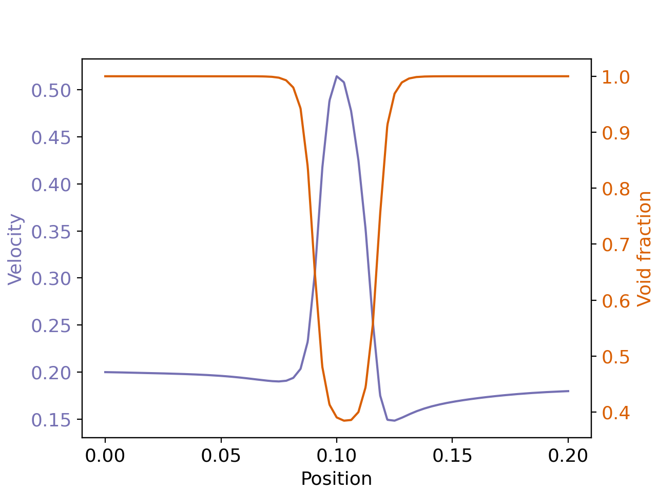
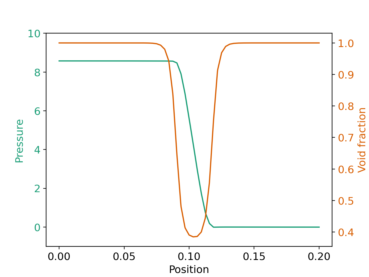
The results are shown in the plots below. We visualise the velocity of the fluid, the void fraction calculated using the particles’ locations, and the pressure drop resulting from the particle-fluid interactions (drag). The plots to the right show the local distribution of the quantities at the center-line of the cylinder.