Sandpile Formation

This example simulates the formation of a sandpile using the discrete element method (DEM). It is based on the simulation of Ai et al. [1], meant to reproduce the 2D photoelastic sandpile experiments led by Zuriguel et al. [2]. More information regarding the DEM parameters is given in the Lethe documentation, i.e. DEM parameters.

Features

• Solvers: lethe-particles

• Two-dimensional problem

• Bi-dispersed particles

• Floating wall

• Post-processing using Python, PyVista, lethe_pyvista_tools, and ParaView.

Files Used in This Example

All files mentioned below are located in the example’s folder (examples/dem/2d-sandpile-formation).

• Geometry file: sandpile.geo

• Mesh file: sandpile.msh

• Parameter files: sandpile-epsd.prm, sandpile-constant.prm, sandpile-viscous.prm

• Post-processing Python scripts: sandpile-postprocessing.py, sandpile-height-comparison.py

Description of the Case

In the first stage of the simulation (\(0-4.5\) s), particles are filled into the hopper. Then, at \(4.5\) s, particles are discharged through a narrow channel onto a flat surface where a pile is formed. We compare the evolution of the height of the pile for the different rolling resistance models with the results obtained by Ai et al. [1]. The angle of repose is also calculated, so as to be compared to the one from the experiment conducted by Zuriguel et al. [2]. We expect that the Elastic-Plastic Spring-Dashpot (EPSD) model will give closer results to the height and angle from the experiment than the viscous model or the constant torque model. Indeed, the constant torque model produces an oscillation that can prevent the pile from reaching a stable state and the viscous model is not adapted here as the viscous effects are not sufficient to stabilize the pile at its real height.

Parameter File

Mesh

The mesh is a hopper with 50.5° angle generated with GMSH, with a channel connecting the hopper to the part with the flat surface. The geometry follows the one used by Zuriguel et al. [2] and the mesh generated with gmsh is structured.

subsection mesh
  set type                = gmsh
  set file name           = ./sandpile.msh
  set check diamond cells = true
  set initial refinement  = 1
end

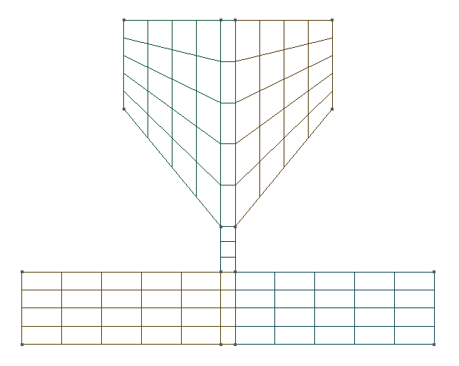
2D mesh of the hopper

Note

The mesh can be generated using the following line:

gmsh -2 sandpile.geo

Lagrangian Physical Properties

The \(3000\) particles are bi-dispersed, with \(2500\) having a diameter of \(6.9\) mm and \(500\) having a diameter of \(8.9\) mm.

The following properties are chosen according to the Ai et al. paper:

• Custom distribution of disks with \(70%\) of disks with a \(6.9\) mm diameter and \(30%\) with an \(8.9\) mm diameter

• Density (\(1056\;\text{kg}/\text{m}^3\))

• Young’s modulus (\(4\) MPa)

• Poisson’s ratio (\(0.49\))

• Friction coefficient of particle-particle (\(0.8)`\)

• Rolling resistance coefficient of particle-particle (\(0.3\))

The same properties were given to the wall as they were not specified in the original article.

subsection lagrangian physical properties
  set g                        = 0.0, -9.81
  set number of particle types = 1
  subsection particle type 0
    set size distribution type            = custom
    set custom diameters                  = 0.0069 , 0.0089
    set custom volume fractions           = 0.7   , 0.3
    set number of particles               = 3000
    set density particles                 = 1056
    set young modulus particles           = 4000000
    set poisson ratio particles           = 0.49
    set restitution coefficient particles = 0.7
    set friction coefficient particles    = 0.8
    set rolling friction particles        = 0.3
  end
  set young modulus wall           = 4000000
  set poisson ratio wall           = 0.49
  set restitution coefficient wall = 0.7
  set friction coefficient wall    = 0.8
  set rolling friction wall        = 0.3
end

Note

Only the value of the restitution coefficient was not given in the reference paper but it did not impact much the height of the pile.

Model Parameters

subsection model parameters
  subsection contact detection
    set contact detection method                = dynamic
    set dynamic contact search size coefficient = 0.8
    set neighborhood threshold                  = 1.3
  end
  set particle particle contact force method = hertz_mindlin_limit_overlap
  set particle wall contact force method     = nonlinear
  set integration method                     = velocity_verlet
  set rolling resistance torque method       = epsd_resistance
  set f coefficient                          = 0.0
end

Note

The f coefficient is only specified when the EPSD rolling resistance model is selected, in this case in prm file sandpile-epsd.prm.

In sandpile-viscous.prm and sandpile-constant.prm, the rolling resistance torque method is set to viscous_resistance and constant_resistance, respectively.

More information regarding the DEM model parameters is given in the Lethe documentation, i.e. DEM Model Parameters.

Particle Insertion

Particles are inserted in an insertion box in the upper part of the hopper. In this simulation, the hopper is filled through 12 insertion steps.

subsection insertion info
  set insertion method                               = volume
  set inserted number of particles at each time step = 250
  set insertion frequency                            = 10000
  set insertion box points coordinates               = -0.34, 0.7 : 0.34, 1.2
  set insertion distance threshold                   = 1.5
  set insertion maximum offset                       = 0.1
  set insertion prn seed                             = 20
end

Note

Due partly to the bi-dispersed particle size distribution, changing the prn seed to a different value can lead to different results since it changes the initial configuration of the particles.

Simulation Control

The simulation runs for 50 seconds of real time. We output the simulation results every 1000 iterations.

subsection simulation control
  set time step        = 2e-5
  set time end         = 50
  set log frequency    = 1000
  set output frequency = 1000
  set output path      = ./output_epsd/
  set output name      = sandpile_epsd
end

Note

To compare with the results of Ai et al., the end time should be set at 50 s or at least 35 s to see the progression of the curve. It can be reduced to 15 s to see the fully formed sandpile but the height of the pile is only measured after 10 s and may continue to decrease after 15 s, particularly with the constant rolling resistance model.

Floating Wall

The floating wall is a temporary flat wall, used here to hold the particles in the hopper during the filling stage, from 0 to \(4.5\) s. It is located at the bottom of the hopper, before the channel.

subsection floating walls
  set number of floating walls = 1
  subsection wall 0
    subsection point on wall
      set x = 0
      set y = 0
    end
    subsection normal vector
      set nx = 0
      set ny = 1
    end
    set start time = 0
    set end time   = 4.5
  end
end

Running the Simulation

The simulation for each rolling resistance model can be launched with

 mpirun -np 2 lethe-particles sandpile-epsd.prm

 mpirun -np 2 lethe-particles sandpile-constant.prm

 mpirun -np 2 lethe-particles sandpile-viscous.prm

Note

If the end time is set at \(50\) s, this example needs a simulation time of approximately 25 minutes on 2 cores, for each of the three rolling resistance models.

Post-processing

A Python post-processing code called sandpile-postprocessing.py is provided with this example. It is used to measure the height of the pile at each time set, starting at \(10.02\) s so that the pile is already formed. It also calculates the angle of repose of the pile, based on the last frame. It compares the data generated by the simulation to the one from Ai et al. [1] for the selected rolling resistance model.

It is possible to run the post-processing code with the following line. The arguments are the simulation path and the rolling resistance model used.

  python3 sandpile-postprocessing.py  --folder ./ --rollingmethod epsd

Important

You need to ensure that lethe_pyvista_tools is working on your machine. Click here for details.

Important

The argument –rollingmethod can be either epsd, viscous or constant and corresponds to the rolling resistance torque method selected in each prm file. The argument –regression can be added to plot the least squares regression used to calculate the angle of repose.

The code prints the values of the coefficient of determination \(R^2\), the slope (from the regression), and the angle of repose.

When you have launched the simulation and the post-processing (with the right argument) for each rolling resistance model (constant, epsd, viscous), launch the following to compare the different models.

  python3 sandpile-height-comparison.py

Results

Visualisation with Paraview

The simulation can be visualised using Paraview as seen below.

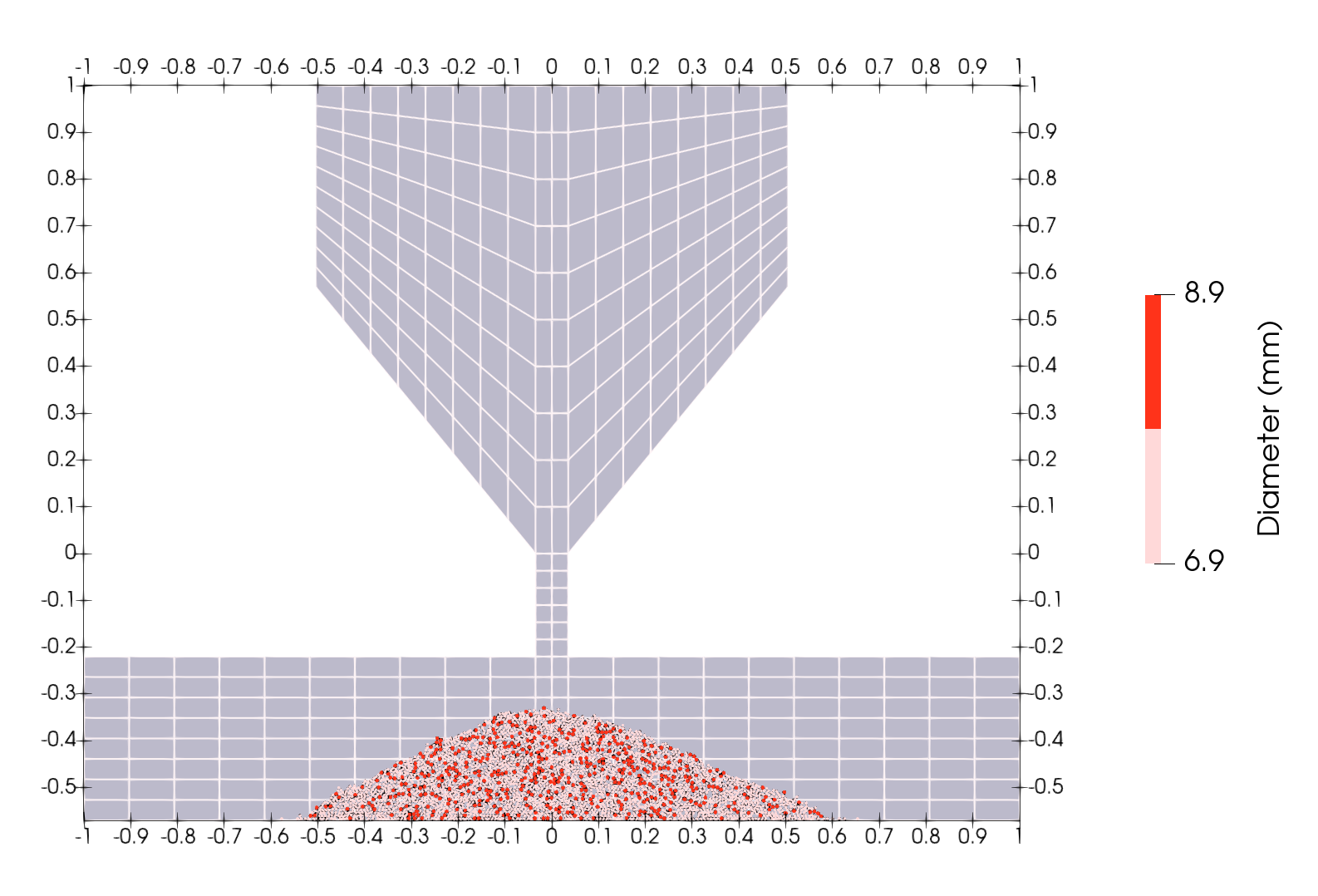
Sandpile at the end of the simulation

Evolution of the Height of the Pile

The following figure compares the evolution of the height of the pile with the results of Ai et al.

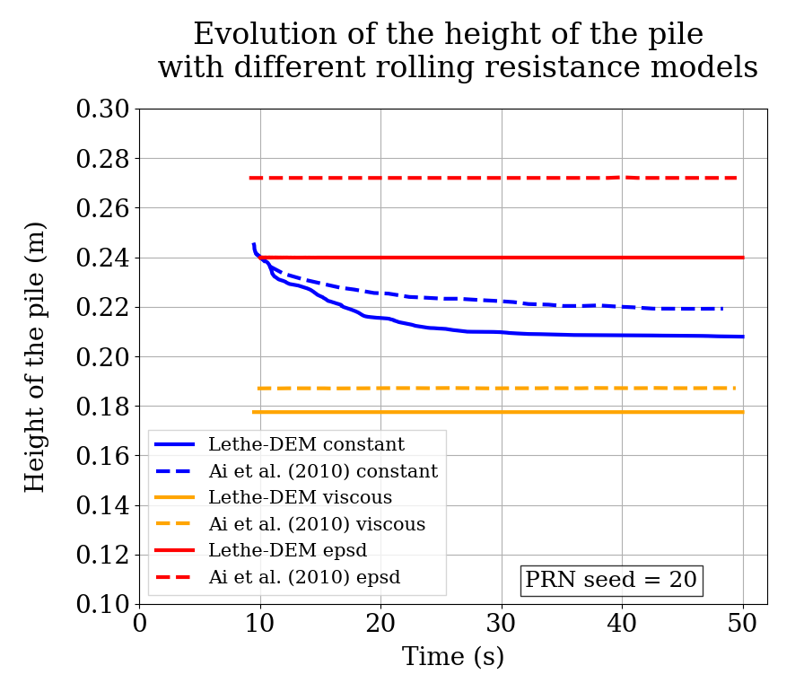
Considering the height of the pile measured in the experiment by Zuriguel et al. was \(28\) cm, the results with model EPSD are satisfying. As predicted, with the constant model, the pile takes a lot of time to stabilize but results are close to those obtained by Ai et al. Regarding the viscous model, the pile does remain constant like with the EPSD model but the height is lower than what is observed in the experiments.

The difference with the Ai et al. simulation could be due to the fact that there are two sizes of particles. As they are inserted, the particles are placed randomly according to the chosen prn seed, which can lead to a difference in the height of the pile.

The next figure shows the evolution of the height of the pile with rolling resistance model EPSD using different PRN seeds.

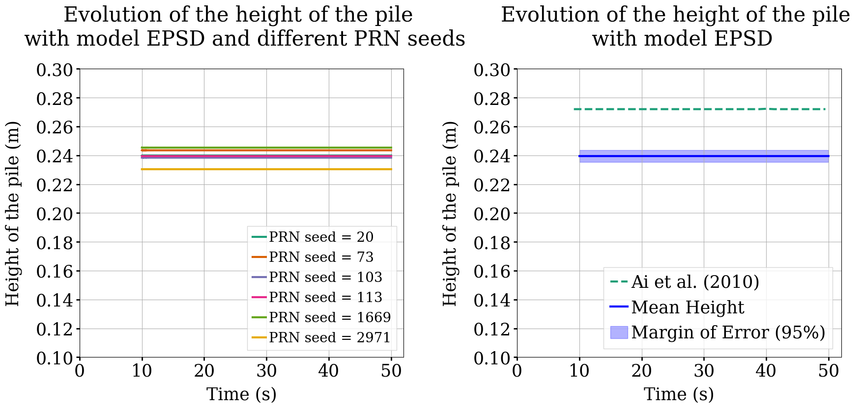
This confirms changing the PRN seed leads to different heights but the results remain around \(24\) cm.

References

[1] (1,2,3)

J. Ai, Jian-Fei Chen, J. Michael Rotter, and Jin Y. Ooi. “Assessment of Rolling Resistance Models in Discrete Element Simulations.” Powder Technology, vol. 206, no. 3, 2011, pp. 269-282. ScienceDirect. [Online]. Available: https://www.sciencedirect.com/science/article/pii/S0032591010005164

[2] (1,2,3)

I. Zuriguel, T. Mullin, J. M. Rotter. “Effect of Particle Shape on the Stress Dip Under a Sandpile.” Physical Review Letters, vol. 98, no. 2, 2007, p. 028001. [Online]. Available: https://journals.aps.org/prl/abstract/10.1103/PhysRevLett.98.028001