Dam-Break

This example simulates the dam break experiments of Martin and Moyce [1].

Features

• Solver: lethe-fluid (with Q1-Q1)

• Two phase flow handled by the Volume of fluids (VOF) approach with interface sharpening

• Unsteady problem handled by an adaptive BDF1 time-stepping scheme

• The use of a python script for post-processing data

Files Used in This Example

Both files mentioned below are located in the example’s folder (examples/multiphysics/dam-break).

• Parameter file: dam-break-Martin-and-Moyce.prm

• Postprocessing Python script: dam-break-2d.py

Description of the Case

A liquid is fixed behind a dam at the left most corner of a rectangular domain as shown in the figure below. At \(t = 0\) s, the dam is removed, and the liquid is released into the total simulation domain.

The following schematic describes the geometry and dimensions of the simulation in the \((x,y)\) plane:

Note

All the four boundary conditions are slip, and an external gravity field of \(-1\) is applied in the \(y\) direction.

Parameter File

Simulation Control

Time integration is handled by a 1st order backward differentiation scheme (bdf1), for a \(4.1\) s simulation time with an initial time step of \(0.01\) seconds.

Note

This example uses an adaptive time-stepping method, where the time-steps are modified during the simulation to keep the maximum value of the CFL condition below a given threshold.

subsection simulation control
  set method           = bdf1
  set time end         = 4
  set time step        = 0.01
  set adapt            = true
  set max cfl          = 0.5
  set output name      = dam-break
  set output frequency = 20
  set output path      = ./output/
end

Multiphysics

The multiphysics subsection enables to turn on (true) and off (false) the physics of interest. Here VOF is chosen.

subsection multiphysics
  set VOF = true
end

Interface Sharpening Parameters

VOF

If the interface sharpening is not enabled in VOF subsection, the interface between phases will become blurry (due to diffusion). Furthermore, the phase filtration is enabled in this example. We refer the reader to the The Volume of Fluid (VOF) Method documentation for more explanation on both methods.

subsection VOF
  subsection interface sharpening
    set enable              = true
    set threshold           = 0.5
    set interface sharpness = 1.5
    set frequency           = 20
  end
  subsection phase filtration
    set type            = tanh
    set beta            = 10
  end
end

Fluid Phase Parameters

Initial Conditions

In the initial conditions, the initial velocity and initial position of the liquid phase are defined. The liquid phase is initially defined as rectangle of length \(= 3.5\) and height \(= 7\).

subsection initial conditions
  set type = nodal
  subsection uvwp
    set Function expression = 0; 0; 0
  end
  subsection VOF
    set Function expression = if (x<3.5 & y<7 , 1, 0)
  end
end

Source Term

The source term subsection defines the gravitational acceleration:

subsection source term
  subsection fluid dynamics
    set Function expression = 0;-1.0; 0
  end
end

Physical Properties

Two fluids are present in this simulation, hence in the physical properties subsection, their physical properties should be defined:

subsection physical properties
  set number of fluids = 2
  subsection fluid 0
    set density             = 1.2
    set kinematic viscosity = 0.01516
  end
  subsection fluid 1
    set density             = 1000
    set kinematic viscosity = 0.000001
  end
end

We define two fluids here simply by setting the number of fluids to be \(2\). In subsection fluid 0, we set the density and the kinematic viscosity for the phase associated with a VOF indicator of 0. Similar procedure is done for the phase associated with a VOF indicator of 1 in subsection fluid 1.

Mesh

We start off with a rectangular mesh that spans the domain defined by the corner points situated at the origin and at point \([14,10]\). The first \(14,10\) couple defines the number of initial grid subdivisions along the length and height of the rectangle. This makes our initial mesh composed of perfect squares. We proceed then to redefine the mesh globally three times by setting set initial refinement=3.

subsection mesh
  set type               = dealii
  set grid type          = subdivided_hyper_rectangle
  set grid arguments     = 14, 10 : 0, 0 : 14, 10 : true
  set initial refinement = 3
end

In the mesh adaptation subsection, adaptive mesh refinement is defined for phase. min refinement level and max refinement level are 3 and 5, respectively. The adaptation strategy fraction type is set to fraction, which leads the mesh adaptation to refine the cells contributing to a certain fraction of the total error. This is highly appropriate for VOF simulations since the error for the VOF field is highly localized to the vicinity of the interface. We set initial refinement steps=4 to ensure that the initial mesh is adapted to the initial condition for the phase.

subsection mesh adaptation
  set type                     = kelly
  set variable                 = phase
  set fraction type            = fraction
  set max refinement level     = 5
  set min refinement level     = 3
  set frequency                = 1
  set fraction refinement      = 0.99
  set fraction coarsening      = 0.01
  set initial refinement steps = 4
end

Running the Simulation

Call lethe-fluid by invoking:

mpirun -np 6 lethe-fluid dam-break-Martin-and-Moyce.prm

to run the simulation using six CPU cores. Feel free to use more.

Warning

The code will compute \(35,000+\) dofs for \(600+\) time iterations. Make sure to compile Lethe in Release mode and run in parallel using mpirun. This simulation takes \(\sim \, 3\) minutes on \(6\) processes.

Results and Discussion

The following image shows the screenshots of the simulation at \(0\), \(1\), \(2\), \(3\), and \(4\) seconds, of the phase results without and with phase filtering. The red area corresponds to the liquid phase and the blue area corresponds to the air phase.

A python post-processing code (dam-break-2d.py) is added to the example folder to post-process the results. Run

python3 ./dam-break-2d.py ./output

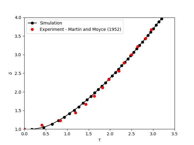
to execute this post-processing code, where ./output is the directory that contains the simulation results. In post-processing, the maximum dimensionless lateral position of the liquid phase is tracked through time and compared with the experiments of Martin and Moyce (1952) [1]. The following figure shows the result of the post-processing, with a good agreement between the simulation and the experiment:

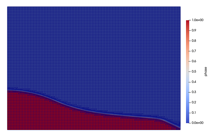
As mentioned previously, this simulation uses adaptive mesh refinement. The following image shows the mesh and the position of the interface at \(4\) s. The mesh refinement detects and refines the meshes on the interface.

References

[1] (1,2)

J. C. Martin et al., “Part IV. An experimental study of the collapse of liquid columns on a rigid horizontal plane,” Philos. Trans. R. Soc. Lond. Ser. Math. Phys. Sci., vol. 244, no. 882, pp. 312–324, Mar. 1952, doi: 10.1098/rsta.1952.0006.