Pseudo-2D Gas-Solid Fluidized Bed

This example simulates the fluidization of a particle bed in gas. It is based on the pseudo-2D experimental setup used by B.G.M. van Wachem et al [1] to validate their two-dimensional fluidized bed simulations.

Features

• Solvers: lethe-particles and lethe-fluid-particles

• Three-dimensional problem

• Gas-solid fluidized bed

• Post-processing using Python, PyVista, lethe_pyvista_tools, and ParaView

Files Used in This Example

All files mentioned below are located in the example’s folder (examples/unresolved-cfd-dem/pseudo-2d-gas-solid-fluidized-bed).

• Parameter file for particle insertion and packing: packing-particles.prm

• Parameter file for CFD-DEM simulation: gas-solid-fluidized-bed.prm

• Geometry file: structure.geo

• Post-processing Python script: fluidized-bed-postprocessing.py

Description of the Case

First, lethe-particles is used to fill the rectangular column with \(17562\) particles, corresponding to the \(39\) g sample of particles used in the experiment. Then, the lethe-fluid-particles solver allows to simulate the fluidization of the particles, with a gas velocity of \(U = 0.9\) m/s at the inlet at the bottom of the column.

DEM Parameter File

All parameter subsections are described in the parameters guide of the documentation.

We first introduce the different subsections of the parameter file packing-particles.prm.

Mesh

The domain is generated with GMSH to reproduce the experimental setup. It is a rectangular column with dimensions \(0.09\times0.008\times0.54\) m.

subsection mesh
  set type                = gmsh
  set file name           = ./structure.msh
  set initial refinement  = 1
end

Simulation Control

A simulation time of \(2.5\) s was chosen, with a time step of \(5\times10^{-6}\). It is important to choose a sufficiently long simulation time so that all particles can become static. The output files generated are stored in the folder output_dem.

subsection simulation control
  set time step        = 0.000005
  set time end         = 2.5
  set log frequency    = 1000
  set output frequency = 1000
  set output path      = ./output_dem/
end

Restart

The lethe-fluid-particles solver requires reading DEM checkpoint files to start the CFD-DEM simulation. These files are written by enabling the checkpoint option in the restart subsection.

subsection restart
  set checkpoint = true
  set frequency  = 10000
  set restart    = false
  set filename   = dem
end

Model Parameters

subsection model parameters
  subsection contact detection
    set contact detection method = dynamic
    set neighborhood threshold   = 1.3
  end
  subsection load balancing
    set load balance method     = dynamic
    set threshold               = 0.5
    set dynamic check frequency = 10000
  end
  set particle particle contact force method = hertz_mindlin_limit_overlap
  set particle wall contact force method     = nonlinear
  set integration method                     = velocity_verlet
end

Lagrangian Physical Properties

In this simulation, \(17562\) particles are inserted, with a diameter of \(1.545\) mm and a density of \(1150\;\text{kg}/\text{m}^3\). The Young’s moduli and poisson ratios are kept to reasonable values. For the friction, restitution and rolling friction coefficients, commonly used values are employed, as suggested in the article. We have observed that the results can be quite dependent on the values of the rolling friction coefficient, which was not specified in the reference article.

subsection lagrangian physical properties
  set g                        = 0, 0, -9.81
  set number of particle types = 1
  subsection particle type 0
    set size distribution type            = uniform
    set diameter                          = 0.001545
    set number of particles               = 17562
    set density particles                 = 1150
    set young modulus particles           = 1e7
    set poisson ratio particles           = 0.3
    set restitution coefficient particles = 0.9
    set friction coefficient particles    = 0.3
    set rolling friction particles        = 0.025
  end
  set young modulus wall           = 1e7
  set poisson ratio wall           = 0.3
  set restitution coefficient wall = 0.9
  set friction coefficient wall    = 0.3
  set rolling friction wall        = 0.025
end

Insertion Info

Particles are inserted within a box in the upper part of the column with the volume insertion method. \(4\) steps are required to insert all the particles.

subsection insertion info
  set insertion method                               = volume
  set inserted number of particles at each time step = 5000
  set insertion frequency                            = 100000
  set insertion box points coordinates               = 0.002, 0.002, 0.15 : 0.089, 0.006, 0.48
  set insertion distance threshold                   = 1.5
  set insertion maximum offset                       = 0.5
  set insertion prn seed                             = 19
end

Floating Walls

To ensure the gas flow is fully developed before reaching the particles, the particle bed needs to be elevated compared to the fluid inlet at the bottom of the column. This is done using a floating wall, with an end time large enough to cover the whole simulation.

subsection floating walls
  set number of floating walls = 1
  subsection wall 0
    subsection point on wall
      set x = 0
      set y = 0
      set z = 0
    end
    subsection normal vector
      set nx = 0
      set ny = 0
      set nz = 1
    end
    set start time = 0
    set end time   = 20
  end
end

Running the DEM Simulation

The packing simulation can be launched on 8 processors with:

mpirun -np 8 lethe-particles packing-particles.prm

Note

Running the packing should take approximately 9 minutes on 8 cores.

After the particles have been packed inside the column, it is now possible to simulate the fluidization of the bed.

CFD-DEM Parameter File

The CFD-DEM simulation is carried out using the lethe-fluid-particles solver and the packed bed generated in the previous stage. The mesh, lagrangian physical properties, DEM model parameters and floating walls subsections are identical to that of the packing parameter file, so they will not be shown here.

Simulation Control

The simulation is run for \(12\) s with a time step of \(0.0002\) s. The time scheme chosen for the simulation is a second-order backward difference method (BDF2).

subsection simulation control
  set method           = bdf2
  set output frequency = 100
  set time end         = 12
  set time step        = 0.0002
  set output path      = ./output/
end

Physical Properties

The kinematic viscosity and density of the gas are set to respectively \(1.33\times10^{-5}\;\text{m}^2/\text{s}\) and \(1.28\;\text{kg}/\text{m}^3\) to match those used in the article.

subsection physical properties
  subsection fluid 0
    set kinematic viscosity = 1.33e-5
    set density             = 1.28
  end
end

Initial Conditions

For the initial conditions, we choose zero initial conditions for the velocity.

subsection initial conditions
  subsection uvwp
      set Function expression = 0; 0; 0; 0
  end
end

Boundary Conditions

For the fluid boundary conditions, the left and right walls (ID = 3) are treated as no-slip boundary conditions, the front and back walls (ID = 2) are defined as slip boundary conditions, the bottom of the column (ID = 0) is an inlet velocity of \(0.9\) m/s and the top of the column (ID = 1) is an outlet for the gas phase. We set the left and the right walls as no-slip boundary conditions to ensure that the gas bubbles is generated in the center of the fluidized bed, as in the experiment.

subsection boundary conditions
  set number = 4
  subsection bc 0
    set id   = 0
    set type = function
    subsection u
      set Function expression = 0
    end
    subsection v
      set Function expression = 0
    end
    subsection w
      set Function expression = 0.9
    end
  end
  subsection bc 1
    set id   = 1
    set type = outlet
  end
  subsection bc 2
    set id   = 2
    set type = slip
  end
  subsection bc 3
    set id   = 3
    set type = noslip
  end
end

Void Fraction

The void fraction calculation uses the checkpoint files from the previous DEM simulation, with the dem prefix. Then, the Quadrature Centered Method (qcm) is employed to carry out the calculation. We set a very small smoothing coefficient of approximatively \(d_p\) to ensure that the void fraction remains bounded. More information about the different methods used to calculate the void fraction is given in the Lethe documentation (Void fraction section).

subsection void fraction
  set mode                         = qcm
  set qcm sphere equal cell volume = true
  set read dem                     = true
  set dem file name                = dem
  set l2 smoothing length          = 0.0015
end

CFD-DEM

We enable all hydrodynamic forces in the CFD-DEM simulation, such as the drag, buoyancy, shear and pressure forces. The drag model used is the Di Felice model, which is a commonly used model for gas-solid flows. We use the default value of the grad-div length scale (grad-div length scale = 1) to ensure that mass conservation is well enforced.

subsection cfd-dem
  set grad div                      = true
  set void fraction time derivative = true
  set drag force                    = true
  set buoyancy force                = true
  set shear force                   = true
  set pressure force                = true
  set drag model                    = difelice
  set coupling frequency            = 100
  set vans model                    = modelA
end

Non-linear Solver

We use the inexact Newton non-linear solver to minimize the number of time the matrix of the system is assembled. This is used to increase the speed of the simulation, since the matrix assembly is computationally expensive.

subsection non-linear solver
  subsection fluid dynamics
    set solver           = inexact_newton
    set tolerance        = 1e-6
    set max iterations   = 20
    set matrix tolerance = 0.2
    set verbosity        = verbose
  end
end

Linear Solver

We use an ILU preconditioner with a fill level of one to ensure that the preconditioner is not too expensive to compute, but that the GMRES method converges adequately.

subsection linear solver
  subsection fluid dynamics
    set method                                = gmres
    set max iters                             = 200
    set relative residual                     = 1e-3
    set minimum residual                      = 1e-11
    set preconditioner                        = ilu
    set ilu preconditioner fill               = 1
    set ilu preconditioner absolute tolerance = 1e-14
    set ilu preconditioner relative tolerance = 1.00
    set verbosity                             = verbose
    set max krylov vectors                    = 200
  end
end

Running the CFD-DEM Simulation

The CFD-DEM simulation is run with the following command:

mpirun -np 10 lethe-fluid-particles gas-solid-fluidized-bed.prm

Note

Running this simulation should take approximately 12 hours on 16 cores.

Post-processing

A Python post-processing code fluidized-bed-postprocessing.py is provided with this example. It is used to compare, at a height of \(45\) mm in the bed, our simulation results with the experimental results obtained by B.G.M. van Wachem et al [1].

The simulation is compared to the experiment using the pressure, void fraction and bed height fluctuations and the power spectral density of the pressure fluctuations. The power spectral density is calculated using the Fast Fourier Transform (FFT) of the pressure fluctuations with a sampling frequency of \(1000\) Hz, and it is then filtered with a Gaussian filter. The Gaussian filter is used to reduce the noise in the pressure signal, by averaging the values with a Gaussian distribution.

The post-processing code can be run with the following command. The argument is the folder which contains the .prm file.

  python3 fluidized-bed-postprocessing.py  --folder ./

Important

You need to ensure that lethe_pyvista_tools is working on your machine. Click here for details.

Results

The following figures compare the pressure, void fraction and bed height fluctuations of the fluidized bed, at \(45\) mm above the floating wall, with the results obtained experimentally by B.G.M. van Wachem et al.

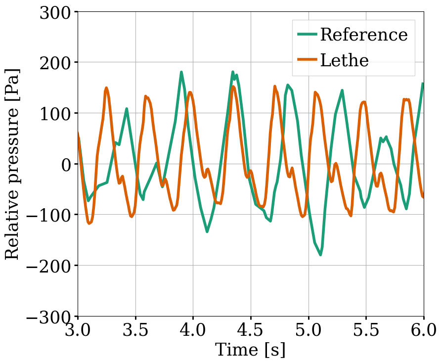
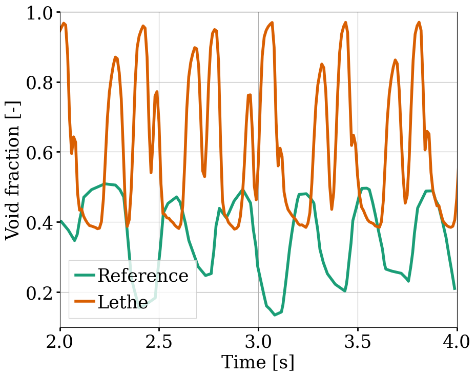
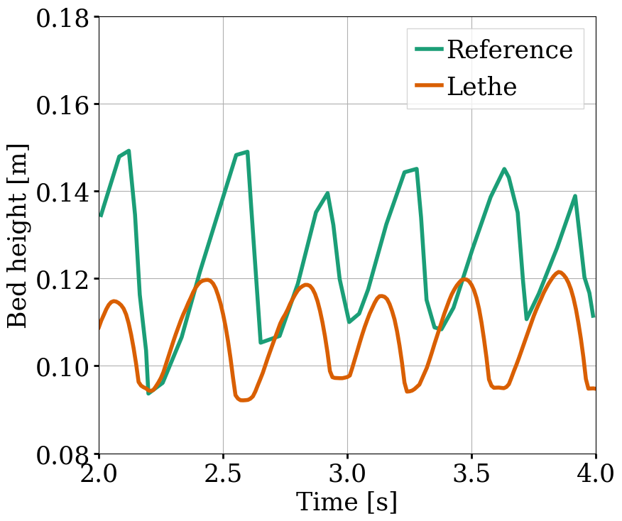
These three figures show that the frequency of the peaks seems to be well replicated for each quantity. However, in the case of the relative pressure and the height of the bed, the amplitude of the signals from the simulation is lower than what was obtained experimentally. Regarding the void fraction, the values are rather far from the experimental ones. This is mainly because the experimental voidage is calculated using light intensity measurements, which can lead to low void fraction values (\(0.2\)). In a packed bed, void fraction is usually higher than \(0.36\).

The following figure compares the simulated pressure power spectral density (PSD) with the one which uses the experimental data.

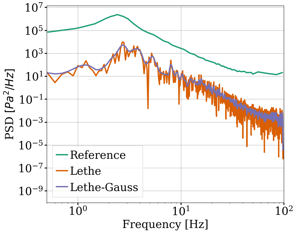
Although the simulation PSD is several orders of magnitude lower, the shape of the curve and the peak frequency show good agreement with the experimental data.

The simulated fluidized bed is shown in the animation below.

Reference

[1] (1,2)

B.G.M. van Wachem, J. van der Schaaf, J.C. Schouten, R. Krishna, and C.M. van den Bleek, “Experimental validation of Lagrangian–Eulerian simulations of fluidized beds,” Powder Technology, vol. 116, pp. 155–165, 2001. Available: https://www.sciencedirect.com/science/article/pii/S0032591000003892.