Inclined 3D Mixer with Pitched-Blade Turbine Impeller Using Composite Sharp-Immersed Boundary#
The mixing in stirred tanks is a common chemical engineering problem that can be tackled through immersed boundary simulation. This example presents an inclined impeller as a variation of 3D Mixer with Pitched-Blade Turbine Impeller Using Composite Sharp-Immersed Boundary to illustrate how to properly define the impeller motion with an arbitrary inclination angle.
Features#
Solvers:
lethe-fluid-sharpTransient problem
Rotating complex solid modeled with an arbitrary inclination with the sharp immersed boundary method
Files Used in This Example#
All files mentioned below are located in the example’s folder (examples/sharp-immersed-boundary/inclined-3d-composite-mixer-with-pbt-impeller).
Composite geometry file:
impeller.compositeParameter file:
mixer.prmPython script for an object rotation angle calculation:
angle_calculator.py
Description of the Case#
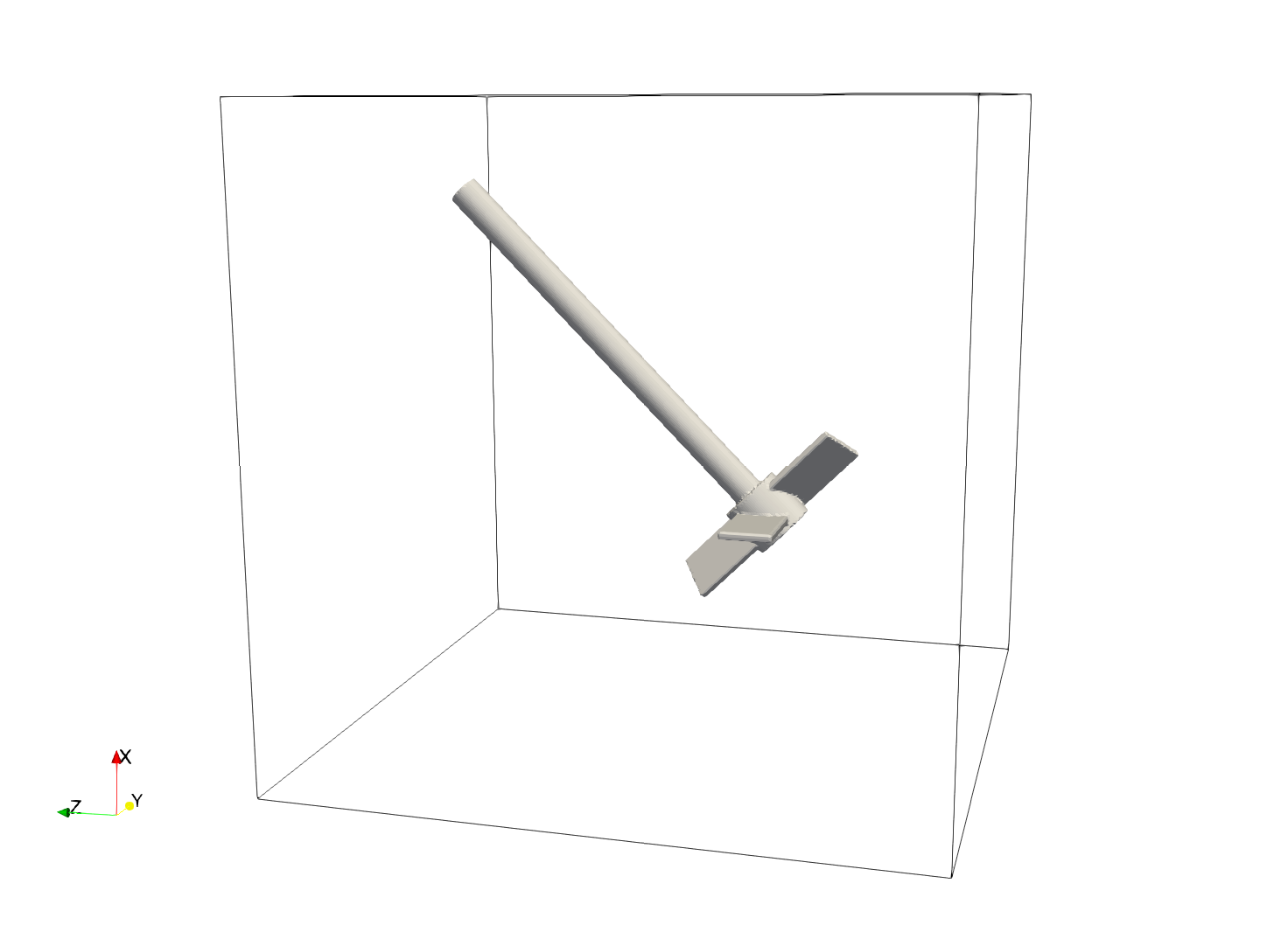
In this example, we simulate a mixer using a PBT impeller through the usage of Sharp-Immersed boundaries. The shape of the impeller is defined by a composition of basic shapes in an identical manner as in example 3D Mixer with Pitched-Blade Turbine Impeller Using Composite Sharp-Immersed Boundary. The objective is to show how to define the rotating motion of the impeller properly when the object is rotating on an arbitrary axis. The tank used in this example is a sample cube. For this case we model an impeller that is rotating around the axis defined by the vector \([1,0,1]\). The visualization of the geometries is presented in the following figure.
Parameter File#
Mesh definition#
The mesh is defined using a simple cube with an initial mesh refinement of 4.
subsection mesh
  set type               = dealii
  set grid type          = subdivided_hyper_rectangle
  set grid arguments     = 1,1,1:-0.5,-0.5,-0.5 : 0.5, 0.5, 0.5: true
  set initial refinement = 4
end
The mesh adaptation is identical to the mesh adaptation section used for the other stirred tanks cases, except that the maximum refinement level has been increased to 8.
subsection mesh adaptation
  set type                 = adaptive
  set error estimator      = kelly
  set variable             = velocity
  set fraction type        = fraction
  set max number elements  = 1200000
  set max refinement level = 8
  set min refinement level = 3
  set frequency            = 1
  set fraction refinement  = 0.2
end
Boundary Conditions#
The boundary condition is similar to the other stirred tank cases, however, the top boundary of the problem is now an open boundary.
subsection boundary conditions
  set number = 6
  subsection bc 0
    set id   = 0
    set type = noslip
  end
  subsection bc 1
    set id   = 1
    set type = noslip
  end
  subsection bc 2
    set id   = 2
    set type = noslip
  end
  subsection bc 3
    set id   = 3
    set type = noslip
  end
  subsection bc 4
    set id   = 4
    set type = noslip
  end
  subsection bc 5
    set id   = 5
    set type = outlet
  end
end
Definition of the Impeller Motion#
The orientation of an object using the sharp interface immersed boundary method is defined using Euler angles and a XYZ rotation convention. As such, determining the orientation of an object as it rotates cannot be directly defined by the direct integration of the angular velocity. Instead use Rodrigues’ rotation matrix (see this link for more details), and from this rotation matrix, we extract the XYZ rotation angle. This calculation can be performed symbolically by a simple Python code using the sympy library. The code is given in the example folder, but is also presented here. Depending on the case, the user needs to study the initial rotation, and angular velocity must be modified. Here, the initial rotation of the impeller is given by a \(\frac{\pi}{4}\) rad rotation around the Y axis to align the impeller with the \([1,0,1]\) vector. Then the rotation speed is given by \(\mathbf{\omega}=2 \pi \frac{\sqrt{2}}{2} [-1,0,-1]\).
from sympy import *
import numpy as np


x, y, z,  ox, oy, oz, pi, t= symbols('x y z ox oy oz pi t ')

def rot_axisx(theta):
    """Returns a rotation matrix for a rotation of theta (in radians) about
    the 1-axis.
    [...]
    """
    ct = cos(theta)
    st = sin(theta)
    lil = ((1, 0, 0),
           (0, ct, -st),
           (0, st, ct))
    return Matrix(lil)


def rot_axisy(theta):
    """Returns a rotation matrix for a rotation of theta (in radians) about
    the 2-axis.
    [...]
    """
    ct = cos(theta)
    st = sin(theta)
    lil = ((ct,0,st),
           (0, 1, 0),
           (-st, 0, ct))
    return Matrix(lil)

def rot_axisz(theta):
    """Returns a rotation matrix for a rotation of theta (in radians) about
    the 3-axis.
    [...]
    """
    ct = cos(theta)
    st = sin(theta)
    lil = ((ct, -st, 0),
           (st, ct, 0),
           (0, 0, 1))
    return Matrix(lil)


def rotation_matrix_to_xyz_angles(R):
    """
    Extracts XYZ rotation angles from a given rotation matrix.

    Parameters:
    R (Matrix): A 3x3 rotation matrix.

    Returns:
    tuple: A tuple of rotation angles (theta_x, theta_y, theta_z) in radians.
    """
    if R.shape != (3, 3):
        raise ValueError("Input must be a 3x3 matrix.")

    # Calculating the angles
    theta_x = atan2(-R[1, 2], R[2, 2])
    theta_y = asin(R[0, 2])
    theta_z = atan2(-R[0, 1], R[0, 0])

    return theta_x, theta_y, theta_z


# Rotation matrix for a small time step dt
initial_rot_x=0
initial_rot_y=pi/4
initial_rot_z=0

Initial_rotation=rot_axisx(initial_rot_x)*rot_axisy(initial_rot_y)*rot_axisz(initial_rot_z)

# Angular velocity vector
ox=-1*np.pi*2*np.sqrt(2)/2.0
oy=0
oz=-1*np.pi*2*np.sqrt(2)/2.0

# Magnitude of the angular velocity vector
omega_mag = sqrt(ox**2 + oy**2 + oz**2)

# Unit vector along the direction of angular velocity
u_x = ox / omega_mag
u_y = oy / omega_mag
u_z = oz / omega_mag

# Rodrigues' rotation formula components
K = Matrix([[0, -u_z, u_y],
            [u_z, 0, -u_x],
            [-u_y, u_x, 0]])

I = Matrix([[1, 0, 0],
            [0, 1, 0],
            [0, 0, 1]])


R = I + sin(omega_mag*t) * K + (1 - cos(omega_mag*t)) * K**2


theta_x, theta_y, theta_z=rotation_matrix_to_xyz_angles(R*Initial_rotation)

# Print orientation
print(str(theta_x).replace("**","^")+';'+str(theta_y).replace("**","^")+';'+str(theta_z).replace("**","^"))
From this Python code, we obtained the following expression of the orientation using the XYZ rotation convention of the impeller as it rotates:
subsection orientation
    set Function expression = atan2(0.707106781186548*sin(pi/4)*sin(6.28318530717959*t) - 0.707106781186548*sin(6.28318530717959*t)*cos(pi/4), (0.5 - 0.5*cos(6.28318530717959*t))*sin(pi/4) + (0.5*cos(6.28318530717959*t) + 0.5)*cos(pi/4));asin((0.5 - 0.5*cos(6.28318530717959*t))*cos(pi/4) + (0.5*cos(6.28318530717959*t) + 0.5)*sin(pi/4));atan2(-0.707106781186548*sin(6.28318530717959*t), -(0.5 - 0.5*cos(6.28318530717959*t))*sin(pi/4) + (0.5*cos(6.28318530717959*t) + 0.5)*cos(pi/4))
end
The parameters used to define the impeller are based on the 3D Mixer with Pitched-Blade Turbine Impeller Using Composite Sharp-Immersed Boundary example and are given as follows:
subsection particles
  set number of particles                     = 1
  set assemble Navier-Stokes inside particles = false
  subsection extrapolation function
    set stencil degree = 2
    set length ratio  = 3
  end
  subsection local mesh refinement
    set initial refinement                = 6
    set refine mesh inside radius factor  = 0
    set refine mesh outside radius factor = 1.25
  end
  subsection output
    set enable extra sharp interface vtu output field = true
  end
  subsection particle info 0
    subsection position
      set Function expression = 0;0;0
    end
    subsection velocity
      set Function expression = 0;0;0
    end
    subsection orientation
      set Function expression = atan2(0.707106781186548*sin(pi/4)*sin(6.28318530717959*t) - 0.707106781186548*sin(6.28318530717959*t)*cos(pi/4), (0.5 - 0.5*cos(6.28318530717959*t))*sin(pi/4) + (0.5*cos(6.28318530717959*t) + 0.5)*cos(pi/4));asin((0.5 - 0.5*cos(6.28318530717959*t))*cos(pi/4) + (0.5*cos(6.28318530717959*t) + 0.5)*sin(pi/4));atan2(-0.707106781186548*sin(6.28318530717959*t), -(0.5 - 0.5*cos(6.28318530717959*t))*sin(pi/4) + (0.5*cos(6.28318530717959*t) + 0.5)*cos(pi/4))
    end
    subsection omega
      set Function expression = -1*pi*2*sqrt(2)/2;0;-1*pi*2*sqrt(2)/2
    end
    set type            = composite
    set shape arguments = impeller.composite
  end
end
Note that orientation and omega result from the symbolic calculations accomplished using Python.
Other differences are that the initial refinement and the refinement zone are adjusted respectively to 6 and 0 to 1.25 reference length. These values are chosen to guarantee that the refinement zone is big enough to cover the motion of the impeller and avoid interaction of the hanging nodes with the sharp immersed boundary constraints.
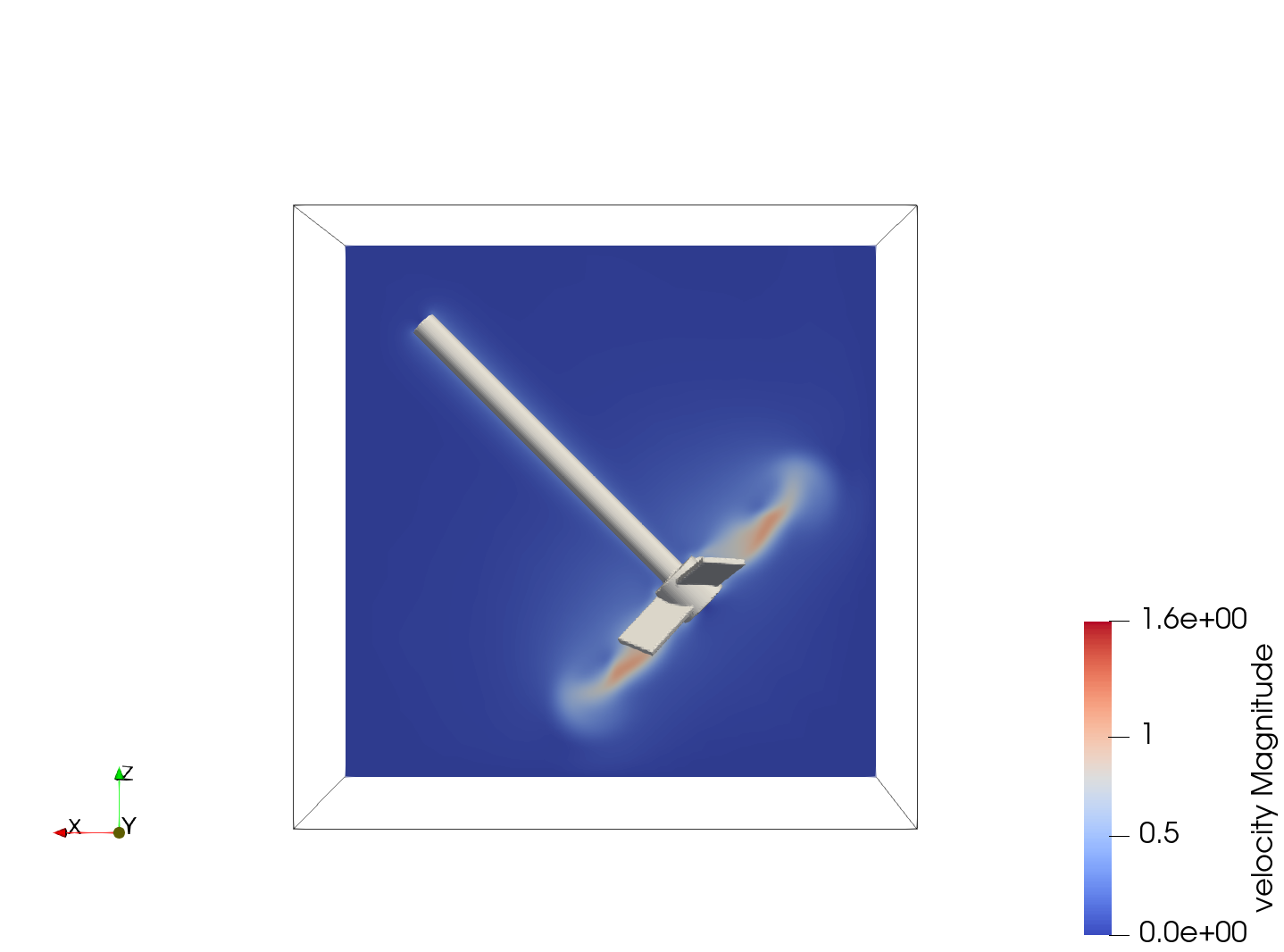
Results#
In the following image the velocity field obtained with this example after 1 second can be observed: