Turbulent Taylor-Couette Flow

This example showcases a turbulent extension of the Taylor-Couette Flow. It features the matrix-free solver (lethe-fluid-matrix-free) which is more computationally efficient when solving problems using high-order elements and fine meshes. It also demonstrates the utilization of initial conditions and the postprocessing of the enstrophy.

Features

• Solvers: lethe-fluid-matrix-free (with Q2-Q2 or Q3-Q3)

• Transient problem using bdf2 time integrator

• Demonstrates the implementation of initial conditions for velocity and pressure

• Demonstrates the postprocessing of the enstrophy

Files Used in This Example

All files mentioned below are located in the example’s folder (examples/incompressible-flow/3d-turbulent-taylor-couette).

• Parameter file: tc-matrix-free.prm

• Reference data files from Wang and Jourdan (2021): [1] (enstrophy_wang_p%.dat)

• Postprocessing Python scripts: tc-postprocessing.py and tc-functions.py

Description of the Case

The Taylor-Couette flow occurs in the annular space between two coaxial cylinders with different angular velocities. For a laminar flow, an analytical solution exists (see Taylor-Couette Flow). As the Reynolds number increases, the flow undergoes a transition where Taylor vortices emerge (symmetrical vortices in the radial-vertical plane). Eventually, as the flow becomes fully turbulent, a chaotic vortex structure appears with intense fluid agitation [2] .

This example is drawn from a case study by Wang and Jourdan [1]. It simulates a turbulent Taylor-Couette flow with a Reynolds number of 4000. It incorporates initial conditions based on a modified version of the laminar solution to generate specific vortical structures, inspired by the Taylor-Green vortex.

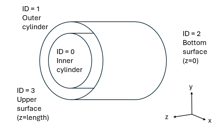
The inner cylinder rotates counterclockwise at a constant angular velocity \(\omega\), while the outer cylinder remains fixed. Periodic boundary conditions are applied to the upper and lower openings of the annular section. The following figure illustrates the geometry of this case:

The initial conditions for velocity and pressure are defined as follow:

\[\begin{split}u_{\theta} &= Ar + \frac{B}{r} + \epsilon U\sin(\theta) \sin \left( \frac{(r-r_i)\pi}{r_i} \right) \sin \left( \frac{z}{d} \right) \\ u_{r} &= \epsilon U\cos(\theta) \sin \left( \frac{(r-r_i)\pi}{r_i} \right) \sin \left( \frac{z}{d} \right) \\ u_{z} &= 0 \\ p &= \frac{1}{2}A^2r^2 + 2AB\ln(r) - \frac{\frac{1}{2}B^2}{r^2} + \frac{1}{2}(\epsilon U)^2 \cos(2\theta) \sin \left( \frac{2(r-r_i)\pi}{r_i} \right) \sin \left( \frac{2z}{d} \right)\end{split}\]

where \(A = -\frac{\omega \kappa^2}{1-\kappa^2}\), \(B = \frac{\omega r_i^2}{1-\kappa^2}\), \(U = \omega r_i\), \(\kappa = \frac{r_i}{r_o}\), \(d = r_o - r_i\), \(\epsilon\) is a relaxing factor, \(r_i\) is the inner cylinder radius, \(r_o\) is the outer cylinder radius, r is the radial coordinate and z is the axial coordinate.

For this particular case, the value for each variable can be found in the following table:

Variable	Value	Variable	Value
A	-0.3333	B	0.3333
U	0.5	\(\kappa\)	0.5
d	0.5	\(\epsilon\)	0.1
\(r_i\)	0.5	\(r_o\)	1.0

Since Lethe uses a Cartesian coordinate system, the following expressions have been transformed to proceed with the simulation. For an incompressible flow, the enstrophy and the kinetic energy are defined as:

\[\begin{split}\mathcal{E} &= \frac{1}{\Omega} \int_{\Omega} \frac{\mathbf{\omega}\cdot \mathbf{\omega}}{2} \mathrm{d}\Omega \\ E_k &= \frac{1}{\Omega} \int_{\Omega} \frac{\mathbf{u}\cdot \mathbf{u}}{2} \mathrm{d}\Omega \\\end{split}\]

where \(\mathbf{\omega}=\nabla \times \mathbf{u}\) represents the vorticity. The results obtained for both enstrophy and kinetic energy are compared to the benchmark values from the case study.

Parameter File

Mesh

The mesh subsection specifies the computational grid:

subsection mesh
  set type               = dealii
  set grid type          = cylinder_shell
  set grid arguments     = 3.14159265359 : 0.5 : 1.0 : 5 : 4 : true
  set initial refinement = 4
end

The type specifies the mesh format used. We use the cylinder_shell from deal.II GridGenerator that creates a shell from two concentric cylinders with the option to set-up specific boundary conditions to each surface. The arguments are the length (3.14159265359), the inner cylinder radius (0.5), the outer cylinder radius (1.0), the number of azimuthal cells (5) and the number of axial cells (4).

The last parameter specifies the initial refinement of the grid. Indicating an initial refinement = 4 implies that the initial mesh is refined 4 times. In 3D, each cell is divided by 8 per refinement. Consequently, the final grid is made of 16 radial elements, 80 azimuthal elements and 64 axial elements for a total of 81,920 cells. The following figure illustrates the mesh:

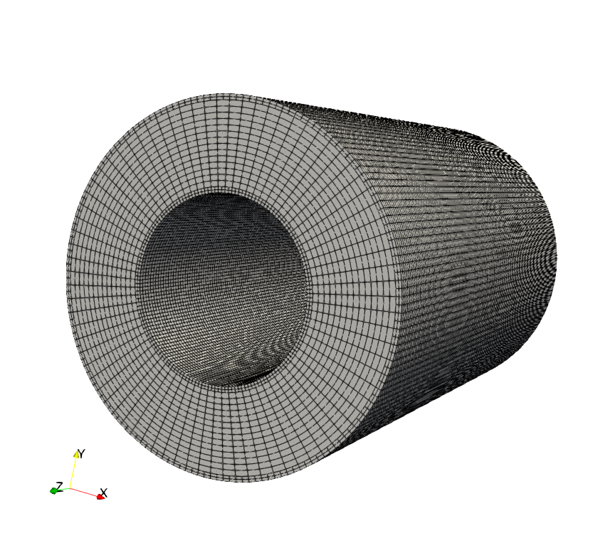
Note

The mesh resolution used in the case study consists of 20 radial elements, 80 azimuthal elements, and 64 axial elements totalling 102,400 elements.

Boundary Conditions

The boundary conditions subsection establishes the constraints on different parts of the domain:

subsection boundary conditions
  set number = 3
  subsection bc 0
    set type = function
    subsection u
      set Function expression = -y
    end
    subsection v
      set Function expression = x
    end
    subsection w
      set Function expression = 0
    end
  end
  subsection bc 1
    set type = noslip
  end
  subsection bc 2
    set type               = periodic
    set id                 = 2
    set periodic_id        = 3
    set periodic_direction = 2
  end
end

First, the number of boundary conditions to be applied must be specified. For each boundary condition, the id of the boundary (refer to geometry for details of surface id) as well as its type must be specified. The inner cylinder (bc 0) is rotating at a constant angular velocity (\(\omega=1 \ \text{rad/s}\)). We use the type = function and prescribe a function for the components of the velocity. By prescribing \(\mathbf{u}=[-y,x,0]^T\), we prescribe the rotation of the inner cylinder at an angular velocity of \(1 \ \text{rad/s}\) in the trigonometric direction. The outer cylinder (bc1) is static and, consequently, a noslip boundary condition is applied. Finally, a periodic condition is used for the inlet and outlet (bc 2). The z- (id=2) is periodic with z+ (id=3). For this condition, the periodic direction must be specified. In Lethe, the periodic direction of 2 implies that the normal direction is the \(\mathbf{e}_z\) vector.

Physical Properties

In the present case, the Reynolds number is defined as: \(Re = \frac{Ud}{\nu}\). Since we set the values of \(U\) and \(d\), the Reynold number of 4000 can be set solely using the kinematic viscosity:

subsection physical properties
  set number of fluids = 1
  subsection fluid 0
    set kinematic viscosity = 6.25e-5
  end
end

Initial Conditions

The initial conditions subsection lets us set-up the velocity and pressure of the flow at \(t = 0 \ \text{s}\):

subsection initial conditions
  set type = nodal
  subsection uvwp
    # A= -(kappa * kappa) / (1. - kappa * kappa);
    # B= ri * ri / (1. - kappa * kappa);
    set Function constants = epsilon=0.1, ri=0.5, omega=1.0, d=0.5 , A= -0.3333333333333333, B= 0.3333333333333333
    set Function expression = cos(atan2(y,x))*(epsilon*omega*ri*cos(atan2(y,x))*sin(((sqrt(x*x+y*y)-ri)*pi)/ri)*sin(z/d)) - sin(atan2(y,x))*(A*(sqrt(x*x+y*y)) + B/(sqrt(x*x+y*y)) + epsilon*omega*ri*sin(atan2(y,x))*sin(((sqrt(x*x+y*y)-ri)*pi)/ri)*sin(z/d)); sin(atan2(y,x))*(epsilon*omega*ri*cos(atan2(y,x))*sin(((sqrt(x*x+y*y)-ri)*pi)/ri)*sin(z/d)) + cos(atan2(y,x))*(A*(sqrt(x*x+y*y)) + B/(sqrt(x*x+y*y)) + epsilon*omega*ri*sin(atan2(y,x))*sin(((sqrt(x*x+y*y)-ri)*pi)/ri)*sin(z/d)); 0.0; ((0.5*A*A*(x*x+y*y)) + (2*A*B*ln(sqrt(x*x+y*y)))) - (0.5*B*B/(x*x+y*y)) + (0.5*(epsilon*omega*ri)*(epsilon*omega*ri)*cos(2*atan2(y,x))*sin((2*(sqrt(x*x+y*y)-ri)*pi)/ri)*sin(2*z/d))
  end
end

The type is set to nodal (as per now, lethe-fluid-matrix-free solver only lets us use this option). Then we choose the uvwp subsection which allows us to respectively set the \(u_x;u_y;u_z;p\) expressions under the function expression. Switching from cylindrical to Cartesian coordinates results in a quite complex expression. To help with that matter, we use the Function constant.

FEM Interpolation

The results obtained for the turbulent Taylor-Couette flow are highly dependent on the numerical dissipation that occurs within the CFD scheme. Generally, high-order methods outperform traditional second-order accurate methods for this type of flow. In the present case, we will compare the usage of second (Q2) and third degree (Q3) polynomial.

subsection FEM
  set velocity order = 2  #3 for Q3
  set pressure order = 2  #3 for Q3
end

Forces

The forces subsection controls the postprocessing of the torque and the forces acting on the boundaries of the domain:

subsection forces
  set verbosity        = quiet   # Output force and torques in log <quiet|verbose>
  set calculate torque = true    # Enable torque calculation
end

By setting calculate torque = true, the calculation of the torque resulting from the fluid dynamics physics on every boundary of the domain is automatically calculated. Setting verbosity = quiet will disable the print out on the terminal for each time step.

Post-processing

subsection post-processing
  set verbosity                        = quiet
  set output frequency                 = 1

  # Kinetic energy calculation
  set calculate kinetic energy         = true
  set kinetic energy name              = kinetic_energy

  # Enstrophy calculation
  set calculate enstrophy              = true
  set enstrophy name                   = enstrophy
end

To monitor the kinetic energy and the enstrophy, we set calculation to true in the post-processing section.

Simulation Control

The simulation control subsection controls the flow of the simulation. To maximize the temporal accuracy of the simulation, we use a second-order bdf2 scheme. Results are written every 10 time-steps. To ensure a more adequate visualization of the high-order elements, we set subdivision = 2. This will allow Paraview to render the high-order solutions with more fidelity.

subsection simulation control
  set method            = bdf2
  set time step         = 0.01
  set adapt             = true
  set max cfl           = 1
  set time end          = 60
  set output frequency  = 10
  set subdivision       = 2
end

Tip

A good practice is to use as many subdivisions as the interpolation order scheme.

Other Subsections

The non-linear solver and linear solver subsections use the same parameters as the Taylor-Green Vortex example. More details can be found in this example and a complete overview of the lethe-fluid-matrix-free linear solver can be found in the Theory Guide (under construction).

Running the Simulation

Launching the simulation is as simple as specifying the executable name and the parameter file. Assuming that the lethe-fluid-matrix-free executable are within your path, the matrix-free simulation can be launched by typing:

mpirun -np n_proc lethe-fluid-matrix-free tc-matrix-free.prm

Results and Discussion

The flow patterns generated by the Taylor-Couette flow are quite complex. The following animation displays the evolution of velocity magnitude on the radial-vertical plane (left) and the Q-criterion iso-contours (right), illustrating the vortical structure as the vortex breaks down and generates smaller structures.

Using the enstrophy.dat file generated by Lethe, the history of enstrophy can be monitored and compared to the reference values extracted from the case study. Assuming that the file is in the same directory as the post-processing scripts, a plot comparing our simulation results to the reference enstrophy data will be generated by using the following command:

python3 tc_postprocessing.py

The enstrophy plot features a zoomed section of the enstrophy cascade. The following plot shows the history of the enstrophy as measured with the Q2 scheme:

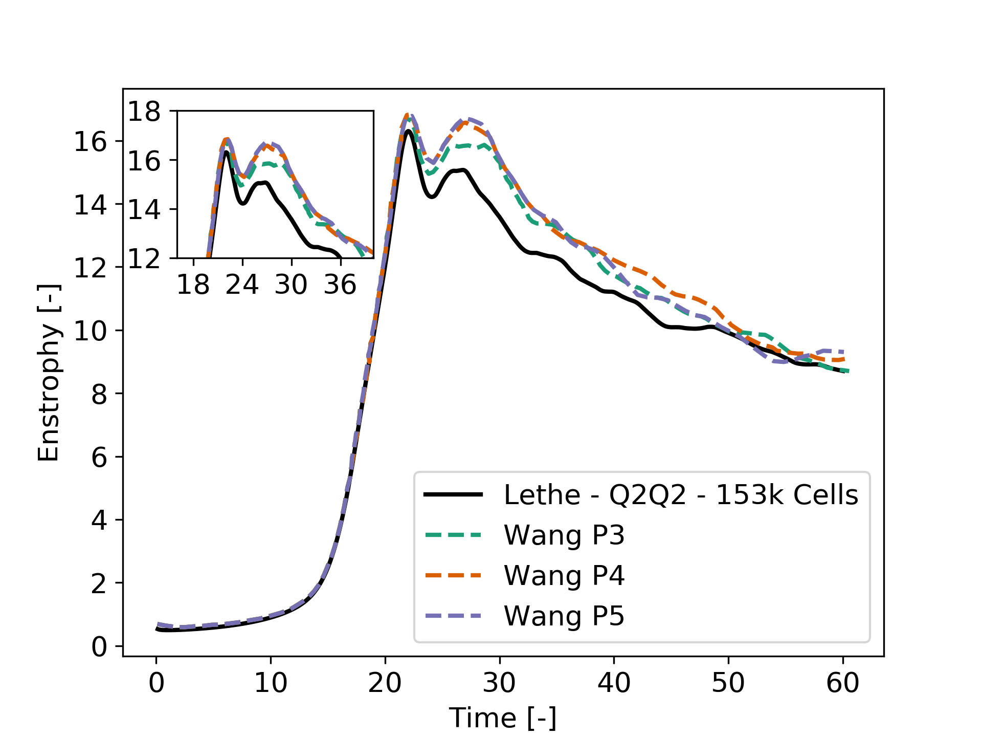
We note that the enstrophy history does not match either reference scheme. Increasing the order from Q2 to Q3 leads to the following results, which are quite close to the P4 and P5 solutions, especially considering that our mesh has about 20% fewer elements:

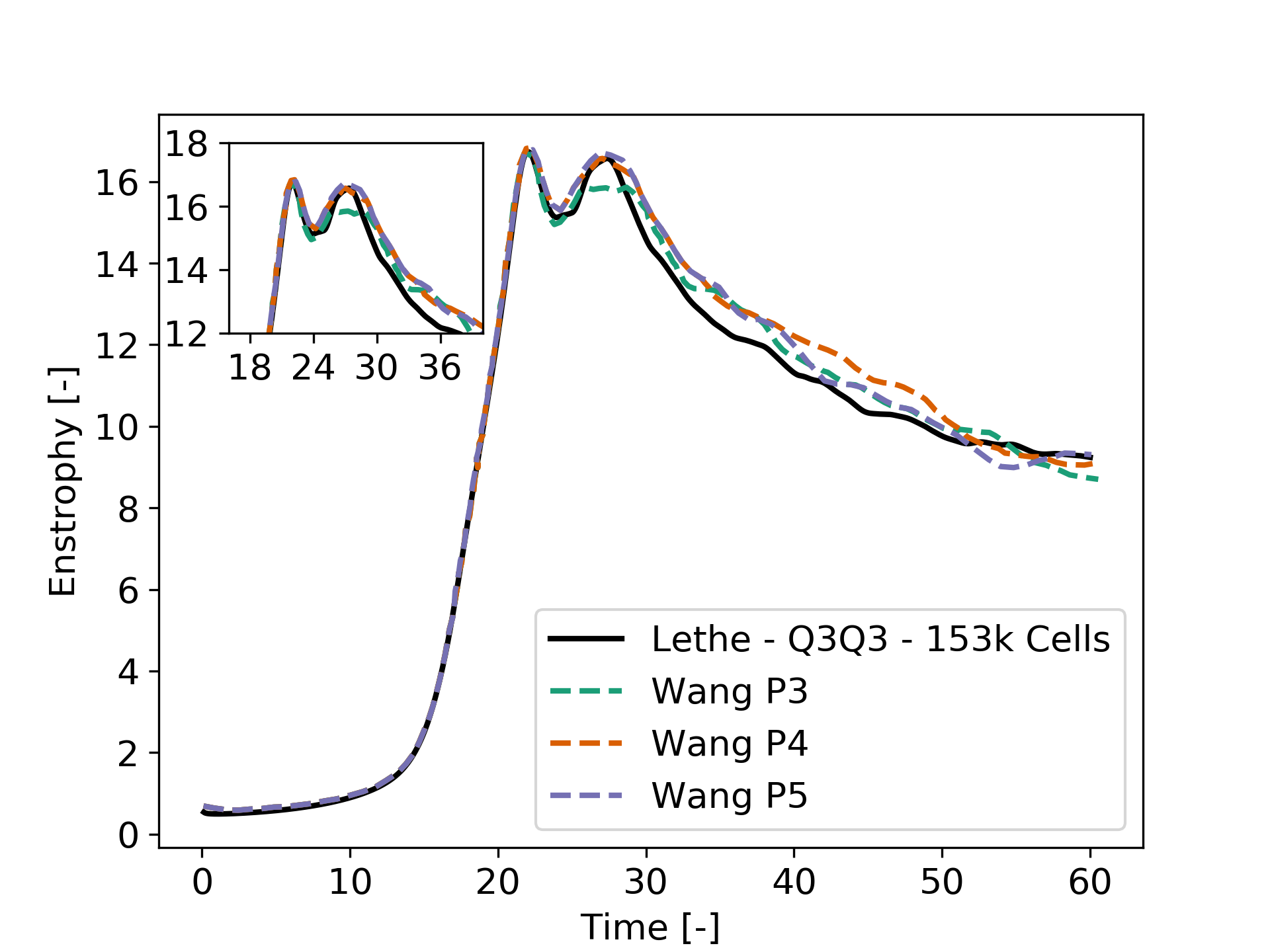
We then revert the scheme order back to Q2 and refine the mesh by setting the initial refinement = 5 in the mesh subsection resulting in a total of 655,360 cells. While this simulation closely matches the references, we observe that the second peak of enstrophy seems to require higher-order elements to be fully captured:

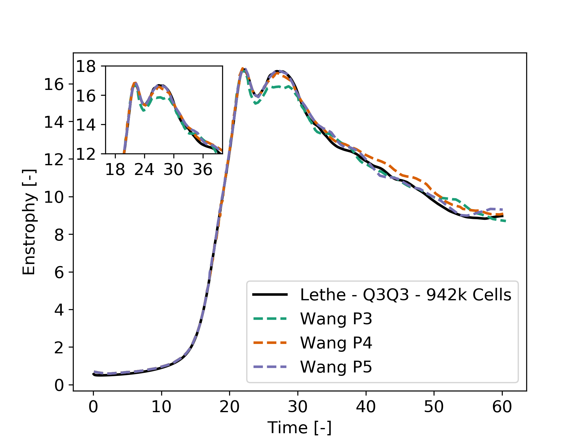
Finally, employing the finer mesh with Q3 elements actually yields a higher second peak of enstrophy and some disparities at the end of the simulation. This could suggest that the results from the case study may not have fully converged yet. Considering one more refinement could be interesting to observe if the solution begins to be mesh-independent:

Possibilities for Extension

• This case offers numerous options for postprocessing. Consider exploring alternative quantities such as vorticity and pressure and use the results to generate interesting animations. Feel free to share them with us!

• It could also be interesting to explore this case with an even higher Reynolds number

References

[1] (1,2)

Z. J. Wang and E. Jourdan, “Benchmark for scale-resolving simulation with curved walls: the Taylor Couette flow,” Advances in Aerodynamics, vol. 3, no. 1, Jun. 2021, doi: 10.1186/s42774-021-00071-0.

[2]

“Taylor–Couette flow,” Wikipedia. Feb. 15, 2024. Available: https://en.wikipedia.org/wiki/Taylor%E2%80%93Couette_flow.