Sloshing in a Rectangular Tank

This example simulates the damping of a small amplitude wave for Reynolds number of (\(2\), \(20\), \(200\) and \(2000\)). The problem is inspired by the test case of Carrica et al. [1]

Features

• Solver: lethe-fluid

• Volume of fluid (VOF)

• Unsteady problem handled by an adaptive BDF2 time-stepping scheme

• Usage of a python script for post-processing data

Files Used in This Example

All files mentioned below are located in the example’s folder (examples/multiphysics/sloshing-in-rectangular-tank).

• Analytical data for \(Re=2\): sloshing_0002/analytical_solution_Re2.csv

• Analytical data for \(Re=20\): sloshing_0020/analytical_solution_Re20.csv

• Analytical data for \(Re=200\): sloshing_0200/analytical_solution_Re200.csv

• Parameter file for \(Re=2\): sloshing_0002/sloshing-in-rectangular-tank_Re0002.prm

• Parameter file for \(Re=20\): sloshing_0020/sloshing-in-rectangular-tank_Re0020.prm

• Parameter file for \(Re=200\): sloshing_0200/sloshing-in-rectangular-tank_Re0200.prm

• Parameter file for \(Re=2000\): sloshing_2000/sloshing-in-rectangular-tank_Re2000.prm

• Postprocessing Python script: sloshing_postprocessing.py

Description of the Case

Predicting the dynamics of free surface waves is essential for many industrial applications (e.g. transport of liquified natural gas). Yet, simulating their dynamics is difficult, especially for high Reynolds number values. Indeed, in this case, the amplitude of the waves dampen very slowly. This leads to an oscillatory wave problem which is highly sensitive to the time integration scheme and the coupling between the VOF solver and the Navier-Stokes solver.

In this problem, we simulate the damping of a small amplitude wave in a rectangular cavity defined from \((-1,-1)\) to \((1,0.1)\). The initial height of the wave \(\xi (x)\) is given by:

\[\xi = 1+0.01 \ sin(\pi(x+0.5))\]

Initial height of the wave

Four values of the Reynolds number are investigated: \(2\), \(20\), \(200\) and \(2000\).

Parameter File

Simulation Control

The results for this problem are highly sensitive to the accuracy of the time-stepping scheme. For this reason, we use a 2nd order backward differentiation scheme (bdf2) with a variable time step. The adaptive time step scaling is set to \(1.025\) to ensure that the time-step does not rise too quickly during wave oscillations.

subsection simulation control
  set method                       = bdf2
  set time end                     = 50
  set time step                    = 0.01
  set adapt                        = true
  set max cfl                      = 0.25
  set output name                  = sloshing-in-rectangular-tank_Re20
  set output path                  = ./output_Re20/
  set output frequency             = 1
  set adaptative time step scaling = 1.025
end

Multiphysics

The multiphysics subsection is used to enable the VOF solver.

subsection multiphysics
  set VOF  = true
end

Initial Conditions

In the initial conditions, we define the initial height of the wave, such that the interface (\(\phi = 0.5\) isocurve) lies at the right height.

subsection initial conditions
  set type = nodal
  subsection uvwp
    set Function expression = 0; 0; 0
  end
  subsection VOF
    set Function expression =  if (y<=(0.01*sin(3.1416*(x+0.5))), min(0.5-(y-0.01*sin(3.1416*(x+0.5)))/0.0025,1), max(0.5-(y-0.01*sin(3.1416*(x+0.5)))/0.0025,0))
  end
end

Mesh

In the mesh subsection, we define a hyper rectangle with appropriate dimensions. The mesh is initially refined 6 times to ensure adequate definition of the interface.

subsection mesh
  set type               = dealii
  set grid type          = subdivided_hyper_rectangle
  set grid arguments     = 5, 2 : -1, -1 : 1, 0.1 : true
  set initial refinement = 6
end

Physical Properties

The physical properties are mainly used to establish the Reynolds number of the sloshing liquid. For the air, however, the work of Carrica et al. [1] does not give any physical properties. We thus fix the air to be significantly less dense than the liquid, but we keep its viscosity at a certain reasonable viscosity to ensure numerical stability.

subsection physical properties
  set number of fluids = 2
  subsection fluid 0
    set density             = 0.001
    set kinematic viscosity = 0.001
  end
  subsection fluid 1
    set density             = 1
    set kinematic viscosity = 0.5
  end
end

Source Term

The source term subsection is used to enable the gravitational acceleration along the \(y\) direction.

subsection source term
  subsection fluid dynamics
    set Function expression = 0 ; -1 ; 0
  end
end

Running the Simulation

We can call lethe-fluid for each Reynolds number. For \(Re=20\), this can be done by invoking the following command:

mpirun -np 8 lethe-fluid sloshing-in-rectangular-tank_Re0020.prm

to run the simulation using eight CPU cores. Feel free to use more.

Warning

Make sure to compile Lethe in Release mode and run in parallel using mpirun. This simulation takes \(\sim \, 8\) minutes (\(Re=2\)) to \(6\) hours (\(Re=2000\)) on \(8\) processes.

Results

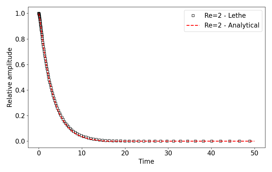
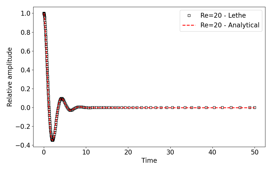
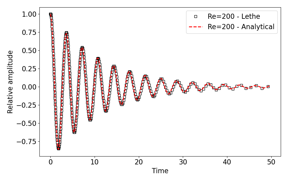
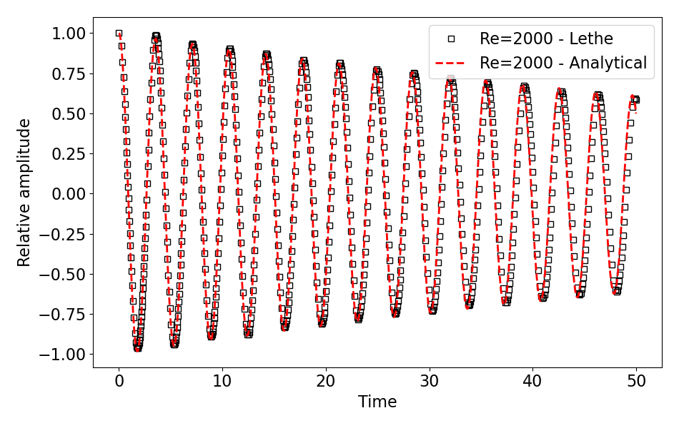
We compare the relative height of the free surface at \(x=0\) with an analytical solution proposed by Wu et al. [2] For the Reynolds number of \(2\), \(20\) and \(200\), data were directly extracted from Carrica et al. [1], whereas for the Reynolds of \(2000\), the simplified analytical expression of Wu et al. [2] is used. The results for Reynolds number of \(2\), \(20\), \(200\) and \(2000\) can be post-processed by invoking the following command from the folder of the Reynolds number of interest (\(Re=20\) in the example below):

python3 ../sloshing_postprocessing.py . sloshing-in-rectangular-tank_Re0020.prm

Important

You need to ensure that the lethe_pyvista_tools is working on your machine. Click here for details.

The following table presents a comparison between the analytical results and the simulation results for all Reynolds numbers mentioned above. A very good agreement is obtained for each of them, demonstrating the accuracy of the VOF solver.

Re	Results
\(2\)
\(20\)
\(200\)
\(2000\)

References

[1] (1,2)

P. M. Carrica, R. V. Wilson, and F. Stern, “An unsteady single-phase level set method for viscous free surface flows,” Int. J. Numer. Methods Fluids, vol. 53, no. 2, pp. 229–256, 2007, doi: 10.1002/fld.1279.

[2] (1,2)

G. X. Wu, R. Eatock Taylor, and D. M. Greaves, “The effect of viscosity on the transient free-surface waves in a two-dimensional tank,” J. Eng. Math., vol. 40, no. 1, pp. 77–90, May 2001, doi: 10.1023/A:1017558826258.