Packing in Ball#
This example is the three-dimensional version of the packing_in_circle example. It is recommended to visit DEM parameters for more detailed information on the concepts and physical meanings of the parameters in Lethe-DEM.
Features#
Solvers:
lethe-particlesThree-dimensional problem
Parallelism
Files Used in This Example#
Parameter file:
examples/dem/3d-packing-in-ball/packing-in-ball.prm
Description of the Case#
Packing in ball example is the three-dimensional version of the packing in circle example.
Warning
The lethe-particles DEM solver in two dimensions is not an accurate model, since several phenomena including torque on particles are intrinsically three-dimensional. Therefore, it should only be used for simple basic analyses before performing three-dimensional simulations.
Parameter File#
The parameter file of packing in ball example is very similar to packing in circle example. We only explain the parts that are different because of the three-dimensional example.
Mesh#
In a three-dimensional simulation, hyper_ball creates a three-dimensional ball (hollow sphere). Note that the first grid argument, which is the center of the triangulation, has three components (0.0, 0.0, 0.0). The expand particle-wall contact search is used in concave geometries to enable particle-wall contact search with boundary faces of neighbor cells for particles located in each boundary cell.
subsection mesh
  set type                                = dealii
  set grid type                           = hyper_ball
  set grid arguments                      = 0.0, 0.0, 0.0 : 0.1 : false
  set initial refinement                  = 3
  set expand particle-wall contact search = true
end
Insertion Info#
In a three-dimensional simulation, we have to define the minimum and maximum dimensions of the insertion box with three components in x, y, and z directions.
subsection insertion info
  set insertion method                               = volume
  set inserted number of particles at each time step = 1000
  set insertion frequency                            = 150000
  set insertion box points coordinates               = -0.05, -0.05, -0.03 : 0.05, 0.05, 0.07
  set insertion distance threshold                   = 2
  set insertion maximum offset                       = 0.75
  set insertion prn seed                             = 19
end
Lagrangian Physical Properties#
Gravitational acceleration has three components in three directions.
subsection lagrangian physical properties
  set g                        = 0.0, 0.0, -9.81
  set number of particle types = 1
  subsection particle type 0
    set size distribution type            = uniform
    set diameter                          = 0.005
    set number of particles               = 5000
    set density particles                 = 2000
    set young modulus particles           = 1e7
    set poisson ratio particles           = 0.3
    set restitution coefficient particles = 0.75
    set friction coefficient particles    = 0.3
  end
  set young modulus wall           = 1e7
  set poisson ratio wall           = 0.3
  set restitution coefficient wall = 0.75
  set friction coefficient wall    = 0.3
end
Model Parameters#
subsection model parameters
  subsection contact detection
    set contact detection method                = dynamic
    set dynamic contact search size coefficient = 0.5
    set neighborhood threshold                  = 1.4
  end
  set particle particle contact force method    = hertz_mindlin_limit_overlap
  set particle wall contact force method        = nonlinear
  set integration method                        = velocity_verlet
end
Simulation Control#
subsection simulation control
  set time step        = 1e-6
  set time end         = 1
  set log frequency    = 10000
  set output frequency = 10000
end
Running the Simulation#
This simulation can be launched by:
We can also launch this simulation in parallel mode. For example, to launch the simulation on 8 processes:
Note
The parallel simulations are generally faster than simulations on a single process. However, to leverage the full performance of a parallel simulation, it should be performed with a load-balancing strategy throughout the simulation. Load-balancing is explained in the next example.
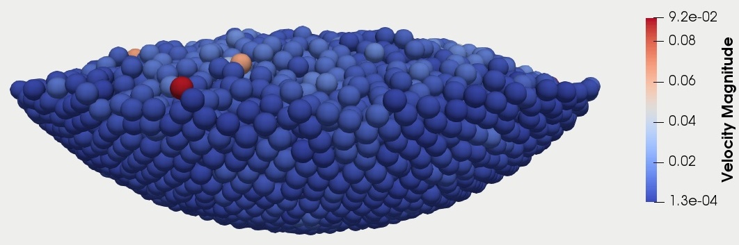
Results#
Packed particles at the end of simulation: