Turbulent Flow Around a Cylinder

This example showcases the turbulent flow around a cylinder at \(Re=3900\). It features the matrix-free solver (lethe-fluid-matrix-free) which is more computationally efficient when solving problems using high-order elements and fine meshes. It also demonstrates the usage of static box refinement and boundary condition refinement to statically refine a mesh.

Features

• Solver: lethe-fluid-matrix-free (with Q1-Q1 and Q2-Q2)

• Transient problem using bdf2 time integrator

• Static mesh refinement using the Box Refinement feature

Files Used in This Example

All files mentioned below are located in the example’s folder (examples/incompressible-flow/3d-turbulent-flow-around-a-cylinder).

• Parameter file: turbulent-cylinder.prm

• Postprocessing Python scripts: postprocess-cylinder.py and cylinder-functions.py

Description of the Case

The flow around bluff bodies such as a cylinder is quite complicated and it is often used as a benchmark problem for CFD. Such flow typically involves boundary-layer separation, flow-regime transition, transition to turbulence, vortex shedding and coherent structures. If the body is symmetric, as is the case for a cylinder, the wake usually exhibits self-induced periodicity from vortices being shed from alternate sides of the body, generating fluctuating forces on the body.

This example is a canonical benchmark for LES, as explained in the book by Grinstein, Margolin and Rider [1]. It also showcases the capabilities of Lethe to statically refine the mesh a the beginning of the simulation using user-defined box refinement. The mesh is refined in the vicinity of the cylinder to capture the boundary layer and the wake region more accurately.

The simulation set-up as well as the boundary ids are illustrated in the following figure:

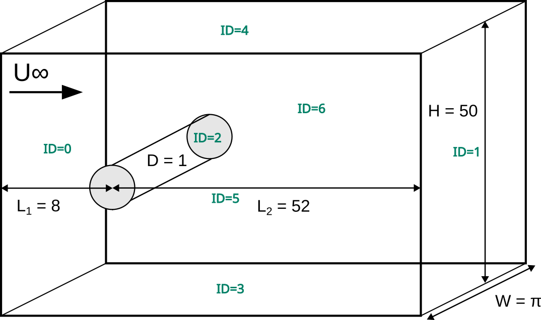
Without loss of generality, \(U_\infty\) is set to 1 and the cylinder diameter \(D\) is set to 1. The Reynolds number is defined as \(Re = \frac{U_{\infty}D}{\nu}\), where \(\nu\) is the kinematic viscosity. The kinematic viscosity is set to \(\nu=2.5641025\times 10^{-4}\), which results in a Reynolds number of 3900.

Parameter File

Mesh

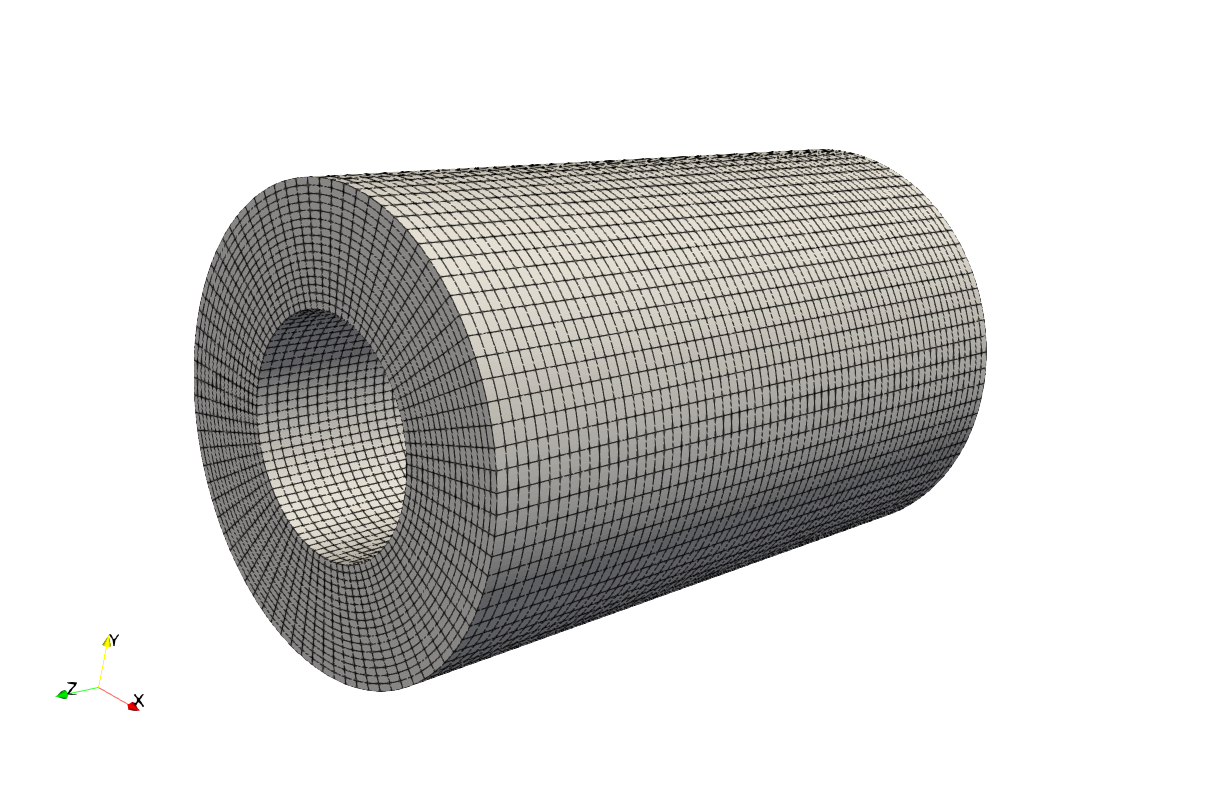
The mesh subsection specifies the computational grid. We use a custom mesh generated using the functionality uniform_channel_with_cylinder of the deal.II library’s GridGenerator to discretize the domain using high-order elements. The mesh is also refined once in the vicinity of the cylinder to capture the boundary layer and wake region more accurately. This is achieved by setting initial boundary refinement = 1 and boundaries refined = 2.

subsection mesh
  set type                        = dealii
  set grid type                   = uniform_channel_with_cylinder
  set grid arguments              = 25 : 8 : 52 : 4.71238898038 : 4 : 0.75 : 5 : 1:  false : true
  set initial boundary refinement = 1
  set boundaries refined          = 2
end

Warning

This uniform_channel_with_cylinder grid generator is only present in the 9.7 version of the deal.II library.

Box refinement

The box refinement subsection refines the mesh in a specific region of the domain. In this case, we refine the mesh around the cylinder to capture the boundary layer and wake region more accurately. The box refinement is defined by its center, size, and refinement level. The mesh is refined by the box refinement twice by setting ìnitial refinement = 2.

subsection box refinement
  subsection mesh
    set type               = dealii
    set grid type          = subdivided_hyper_rectangle
    set grid arguments     = 1, 1, 1 : -2, -3, -1 : 52, 3, 5 : false
    set initial refinement = 0
  end
  set initial refinement = 2
end

A slice of the final mesh obtained from both the initial boundary refinement and the box refinement is shown in the following figure:

Boundary Conditions

The boundary conditions subsection establishes the boundary conditions:

subsection boundary conditions
  set number = 6
  subsection bc 0
    set type = function
    subsection u
      set Function expression = 1
    end
    subsection v
      set Function expression = 0
    end
    subsection w
      set Function expression = 0
    end
  end
  subsection bc 1
   set type = outlet
   set beta = 1
  end
  subsection bc 2
    set type = noslip
  end
  subsection bc 3
    set type = slip
  end
  subsection bc 4
    set type = slip
  end
  subsection bc 5
    set type               = periodic
    set periodic_id        = 6
    set periodic_direction = 2
  end
end

Periodic boundary conditions are applied to the front (id=5) and back (id=6) walls of the domain to mimic an infinite domain along the main axis of the cylinder.

Physical Properties

The Reynolds number is defined as: \(Re = \frac{U_{\infty}D}{\nu}\), where \(U_{\infty}\) is the velocity at the inlet, \(D\) is the cylinder diameter, and \(\nu\) is the kinematic viscosity. Since we set the values of \(U_{\infty}\) and \(D\), the Reynold number of 3900 can be imposed using the kinematic viscosity:

subsection physical properties
  set number of fluids = 1
  subsection fluid 0
    set kinematic viscosity = 2.5641025e-04
  end
end

FEM Interpolation

The results obtained for the turbulent flow around a cylinder are highly mesh and order dependent. The present example consider both \(Q_1Q_1\) and \(Q_2Q_2\) elements. The order of the velocity and pressure interpolation can be set in the FEM subsection.

subsection FEM
  set velocity order = 1
  set pressure order = 1
end

Forces

The forces subsection controls the postprocessing of the torque and the forces acting on the boundaries of the domain:

subsection forces
  set verbosity        = verbose
  set calculate force  = true
  set output precision = 10
  set output frequency = 10
end

By setting calculate force = true, the calculation of the force resulting from the fluid dynamics physics on every boundary of the domain is automatically calculated.

Post-processing

To monitor the average velocity and pressure, we set calculate average velocities = true in the post-processing subsection. The average velocity is computed starting from the time step specified by initial time for average velocity = 25. This allows us to focus on the statistically steady state of the flow.

subsection post-processing
  set calculate average velocities      = true
  set initial time for average velocity = 25
end

Simulation Control

The simulation control subsection controls the flow of the simulation. To maximize the temporal accuracy of the simulation, we use a second-order bdf2 scheme. Results are written every 500 time-steps.

subsection simulation control
  set method           = bdf2
  set output name      = cylinder-Re3900
  set output path      = ./output/
  set time end         = 200
  set adapt            = true
  set max cfl          = 1
  set time step        = 0.002
  set output frequency = 500
end

Running the Simulation

Assuming that the lethe-fluid-matrix-free executable are within your path, the simulation can be launched with the following command:

mpirun -np n_proc lethe-fluid-matrix-free turbulent-cylinder.prm

and choosing the number of processes n_proc according to the resources you have available.

Note

The simulation takes approximatively 10 hours on 16 cores of a AMD Ryzen 9 7950X 16-Core Processor.

Results and Discussion

In the following, results obtained with a box refinement of [2,3,4] levels and using \(Q_1Q_1\) and \(Q_2Q_2\) elements are presented. The results are compared with the literature, including the work of Cardell [2], Ong and Wallace [3], and Norberg [4].

First, the following animation displays the evolution of the velocity magnitude on a slice of the domain over time for a very coarse mesh (\(Q_1Q_1\) with box refinement of 2):

The secondanimation also present the velocity magnitude on the same slice but for a finer mesh and using high-order elements (\(Q_2Q_2\) with box refinement of 3). We we can clearly see much more details in the flow structure, such as the boundary layer and the wake region.

The key validation metrics are:

• Strouhal number:

\[St = \frac{f D}{U_\infty}\]

where \(f\) is the frequency of vortex shedding, \(D\) is the cylinder diameter, and \(U_\infty\) is the free-stream velocity. The frequency of vortex shedding is determined using a Fast Fourier Transform (FFT) of the lift force.

• Drag coefficient:

\[C_d = \frac{F_x}{\frac{1}{2} \rho U_\infty^2 A}\]

where \(F_x\) is the time-averaged x-component of the force at the cylinder wall, \(\rho\) is the fluid density, and \(A\) is the reference area. In this 3D simulation, it is taken as the product of the cylinder diameter and its span in the z-direction.

• Pressure coefficient:

\[C_p = \frac{\bar{p} - p_\infty}{\frac{1}{2} \rho U_\infty^2}\]

where \(\bar{p}\) is the time-averaged pressure and \(p_\infty\) is the reference pressure sampled upstream of the cylinder at the inlet boundary condition.

The drag coefficient, the Strouhal number, and the pressure coefficient are computed using the postprocessing script postprocess-cylinder.py:

python postprocess-cylinder.py -f output -l label

where the -f option specifies the output folder and the -l option specifies the label of the simulation (e.g., Q1Q1 or Q2Q2). This script can be used to visualize a single simulation or to compare multiple simulations by providing a list of folders and labels.

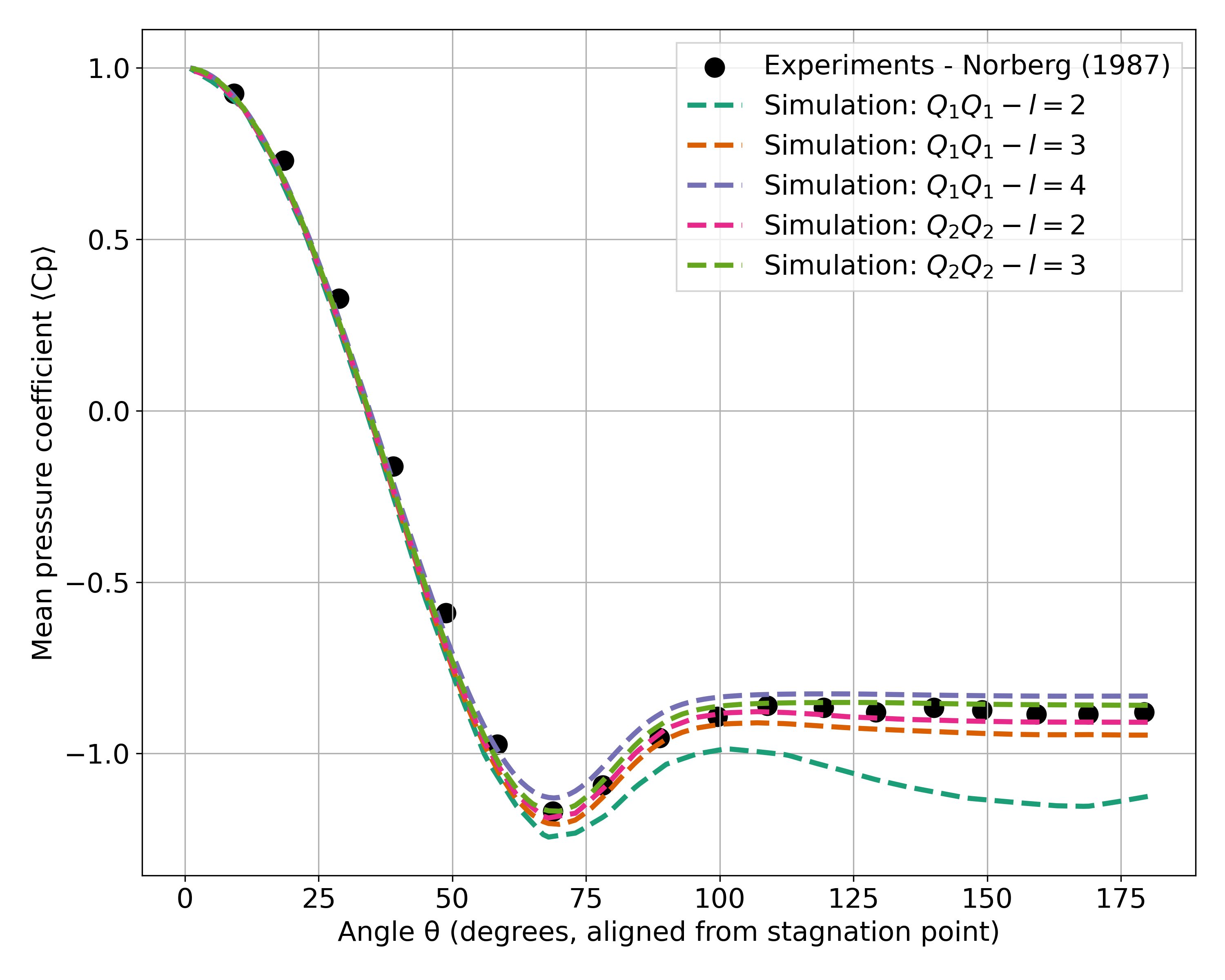
The drag coefficient measured experimentally by Norberg [5] is 1.0075. The Strouhal number value reported by Cardell [2] is \(0.215 \pm 0.005\) and the value reported by Ong and Wallace [3] is \(0.208 \pm 0.002\).

The following table summarizes the results obtained in this example, including the Strouhal number \(S_t\) and the drag coefficient \(C_d\).

Element	Mesh refinement (l)	\(C_d\)	\(S_t\)
\(Q_1Q_1\)	2	1.2105	0.1965
\(Q_1Q_1\)	3	1.0305	0.2110
\(Q_1Q_1\)	4	0.9901	0.2122
\(Q_2Q_2\)	2	1.0008	0.2134
\(Q_2Q_2\)	3	0.9784	0.2112

Finally, we compare the pressure coefficient \(C_p\) obtained in this example with the experimental data from Norberg [5]. The following figure shows the pressure coefficient along the cylinder surface for both \(Q_1Q_1\) and \(Q_2Q_2\) elements, compared to the experimental data:

Possibilities for Extension

• The Reynolds stress tensor and the average velocity downstream of the cylinder can be used to provide additional validation information.

• The case could be extended to a higher Reynolds number, such as \(Re=1.5\cdot 10^5\), as covered in the book by Grinstein, Margolin and Rider [1].

References

[1] (1,2)

6. Grinstein, L. Margolin, W. J. Rider, Implicit large eddy simulation, Cambridge University Press (2007).

[2] (1,2)

G.S. Cardell, Flow past a circular cylinder with a permeable splitter plate, Ph.D. Thesis, Graduate Aeronautical Laboratories, California Institute of Technology, 1993.

[3] (1,2)

10. Ong and L. Wallace, The velocity field of the turbulent very near wake of a circular cylinder, Exp. Fluids 20, 441 (1996).

[4]

3. Norberg, Effects of Reynolds number and a low-intensity freestream turbulence on the flow around a circular cylinder, Publication No. 87/2, Department of Applied Thermodynamics and Fluid Mechanics, Chalmers University of Technology, Gothenburg, Sweden, 1987.

[5] (1,2)

3. Norberg, Experimental investigation of the flow around a circular cylinder: influence of aspect ratio, J. Fluid Mech. 258, 287–316 (1994).