Static Bubble

This example simulates a two-dimensional static bubble [1].

Features

• Solver: lethe-fluid

• Two phase flow handled by the Volume of fluids (VOF) approach with surface tension force

• Calculation of filtered phase fraction gradient and curvature fields

• Unsteady problem handled by a BDF1 time-stepping scheme

Files Used in This Example

Both files mentioned below are located in the example’s folder (examples/multiphysics/static-bubble).

• Parameter file: static_bubble.prm

• Postprocessing Python script: static_bubble.py

Description of the Case

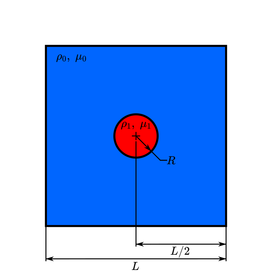
A circular bubble of radius \(R=0.5\) is at equilibrium in the center of a two-dimensional squared domain of side length \(L=5.0\) filled with air. The gravitational force is neglected, such as in a microgravity environment, and the ratio of density between the droplet and the air is 1, meaning that buoyancy is also neglected. Therefore, without any external force, the bubble and the air are at rest, and only the surface tension effects are involved, maintaining the droplet in its circular shape. The following schematic describes the geometry and dimensions of the simulation in the \((x,y)\) plane:

Surface Tension Force

When including the surface tension force in the resolution of the Navier-Stokes equations, the numerical computation of the curvature can give rise to parasitic flows near the interface between the two fluids, as presented in The Volume of Fluid (VOF) Method theory guide.

The static bubble case is a relevant case to study the parasitic currents, since the analytical solution is zero for the velocity. Therefore, non-zero velocities in the computed velocity field are considered parasitic currents [1]. The analytical pressure drop between the interior (\(p_{int}\)) and exterior (\(p_{ext}\)) of the bubble is given by the Young-Laplace relation:

\[\Delta p = p_{int} - p_{ext} = \sigma \kappa\]

with the analytical curvature of the 2D bubble : \(\kappa = 1/R\). This example is based on the static droplet case reported in [1], where \(\sigma = 1.0\), \(R = 0.5\) and \(\kappa = 2.0\).

Parameter File

Simulation Control

Time integration is handled by a 1st order backward differentiation scheme (BDF1), for a \(6~\text{s}\) simulation time with a constant time step of \(0.005~\text{s}\).

subsection simulation control
  set method           = bdf1
  set time end         = 6.0
  set time step        = 0.005
  set output name      = static-bubble
  set output frequency = 20
  set output path      = ./output/
  set subdivision      = 3
end

Multiphysics

The multiphysics subsection enables to turn on (true) and off (false) the physics of interest. Here VOF is chosen. The surface tension force are enabled in the VOF subsection.

subsection multiphysics
  set VOF = true
end

Mesh

The computational domain is defined by a square with opposite corners located at \((-2.5,-2.5)\) and \((2.5,2.5)\). In the mesh subsection, the parameter grid type is set to hyper_rectangle since the discretization is uniform in both direction and the parameter grid arguments defines the opposite corners of the domain. The latter is discretized by an uniform mesh and the refinement level is set to 7 with the parameter initial refinement.

subsection mesh
  set type               = dealii
  set grid type          = hyper_rectangle
  set grid arguments     = -2.5, -2.5 : 2.5, 2.5 : true
  set initial refinement = 7
end

Initial Conditions

In the initial conditions subsection, the initial velocity and initial position of the droplet are defined. The droplet is initially defined as a circle with a radius \(R= 0.5\) in the center of the defined computational domain at \((x,y)=(0.0, 0.0)\). We enable the use of a projection step with diffusion in the subsection projection step to ensure that the initial phase distribution is sufficiently smooth and avoid a staircase representation of the interface. This projection step is implemented in the same way as described in section Normal and Curvature Computations. We refer to the parameter guide Initial Conditions for more details.

subsection initial conditions
  set type = nodal
  subsection uvwp
    set Function expression = 0; 0; 0
  end
  subsection VOF
    set Function expression = if (x^2 + y^2 < 0.5^2 , 1, 0)
    subsection projection step
      set enable           = true
      set diffusion factor = 1
    end
  end
end

VOF

The surface tension force computation is enabled in the VOF subsection. The value of the filter factors \(\alpha\) and \(\beta\) described in section Normal and Curvature Computations are controlled respectively by the parameters phase fraction gradient filter factor and curvature filter factor. Finally, the parameter output auxiliary fields set at true enables the output of the filtered phase fraction gradient and filtered curvature fields.

subsection VOF
  subsection surface tension force
    set enable                                = true
    set phase fraction gradient filter factor = 4
    set curvature filter factor               = 1
    set output auxiliary fields               = true
  end
end

Tip

The phase fraction gradient filter value (\(\eta_n = \alpha h^2\)) and curvature filter value (\(\eta_\kappa = \beta h^2\)) must be small values larger than 0. We recommend the following procedure to choose a proper value for these parameters:

1. Enable output auxiliary fields to write filtered phase fraction gradient and filtered curvature fields.

2. Choose a value close to 1, for example, the default values \(\alpha = 4\) and \(\beta = 1\).

3. Run the simulation and check whether the filtered phase fraction gradient and filtered curvature fields are smooth and without oscillation.

4. If the filtered phase fraction gradient and filtered curvature fields show oscillations, increase the value \(\alpha\) and \(\beta\) to larger values, and repeat this process until reaching smooth filtered phase fraction gradient and filtered curvature fields without oscillations. Generally, the default values should be sufficient.

Physical Properties

The density and the kinematic viscosity of the two fluids involved in this example are set in the subsection physical properties. To neglect buoyancy, the density of both fluids is set to \(10.0\). And, the kinematic viscosity is set to \(0.1\) in both cases. Finally, a fluid-fluid type of material interaction is added to specify the surface tension model. In this case, it is set to constant with the surface tension coefficient \(\sigma\) set to \(1.0\).

subsection physical properties
  set number of fluids = 2
  subsection fluid 1
    set density             = 10
    set kinematic viscosity = 0.1
  end
  subsection fluid 0
    set density             = 10
    set kinematic viscosity = 0.1
  end
  set number of material interactions = 1
  subsection material interaction 0
    set type = fluid-fluid
    subsection fluid-fluid interaction
      set first fluid id              = 0
      set second fluid id             = 1
      set surface tension model       = constant
      set surface tension coefficient = 1
    end
  end
end

Analytical Solution

As presented in the section Surface Tension Force, the analytical solution for this case is zero for the velocity and the pressure drop is given by \(\Delta p = \sigma \kappa\) whit \(\kappa = 1/R\). For \(\sigma = 1.0\) and \(R=0.5\), we have \(\Delta p = 2.0\).

When providing the analytical solution in the analytical solution subsection and setting the parameter enable to true, we can monitor the \(\mathcal{L}^2\) norm of the error on the velocity and pressure fields. They are outputted in the file specified in the parameter filename.

subsection analytical solution
  set enable                = true
  set verbosity             = quiet
  set filename              = L2Error
  subsection uvwp
   set Function expression = 0; 0; if (x^2 + y^2 < 0.5^2 , 2, 0)
  end
end

Running the Simulation

Call the lethe-fluid by invoking:

mpirun -np 8 lethe-fluid static-bubble.prm

to run the simulation using eight CPU cores. Feel free to use more.

Warning

Make sure to compile Lethe in Release mode and run in parallel using mpirun. This simulation takes \(\approx\) 10 mins on 8 processes.

Results and Discussion

Using Paraview, we can visualize the evolution of the velocity field over the time:

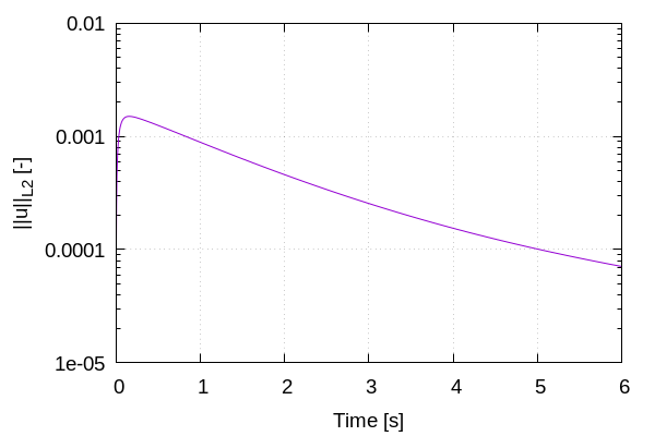
The time evolution of the \(\mathcal{L}^2\) norm of the error on the velocity magnitude is obtained from a Gnuplot script available in the example folder by launching in the same directory the following command:

gnuplot -c "./postprocess.gnu" "./output"

where ./postprocess.gnu is the path to the provided script and ./output is the path to the directory that contains the L2Error.dat file. The figure, named L2Error.png, is outputted in the directory ./output.

Mesh Convergence Study

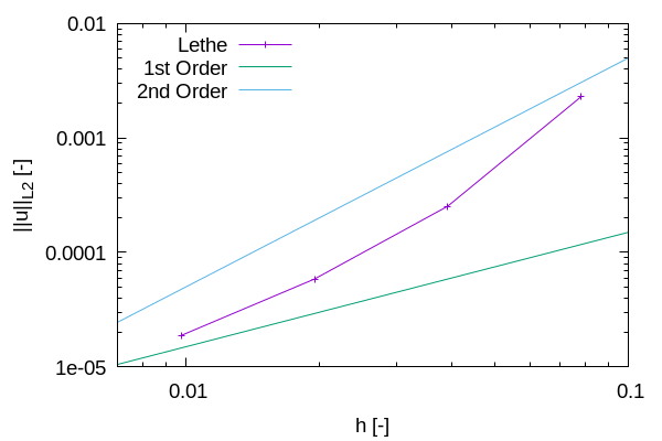
While the filters presented in section Normal and Curvature Computations allow to decrease the magnitude of the parasitic currents, it can be seen from the previous results that they don’t completely disappear. It is, therefore, interesting to see if they vanish with a mesh refinement by performing a space convergence study on their magnitude.

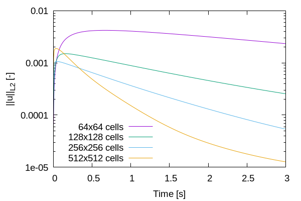
Four levels of refinement are studied (6 to 9) by changing the parameter initial refinement in the mesh subsection. The \(\mathcal{L}^2\) norm of the error on the velocity at 3 seconds is selected as the verification metric. The following figure shows that the scheme reaches nearly an order of accuracy of 2 in space.

Finally, the time evolution of the \(\mathcal{L}^2\) norm of the error on the velocity magnitude for each refinement level can be plotted:

References

[1] (1,2,3)

S. Zahedi, M. Kronbichler, and G. Kreiss, “Spurious currents in finite element based level set methods for two-phase flow,” Int. J. Numer. Methods Fluids, vol. 69, no. 9, pp. 1433–1456, 2012, doi: 10.1002/fld.2643.

[2]

J. U. Brackbill, D. B. Kothe, and C. Zemach, “A continuum method for modeling surface tension,” J. Comput. Phys., vol. 100, no. 2, pp. 335–354, Jun. 1992, doi: 10.1016/0021-9991(92)90240-Y.