Sudden-Expansion Flow

Features

• Solver: lethe-fluid (with Q1-Q1)

• Steady-state and transient solutions

• Comparison with experimental and numerical results

Files Used in This Example

All files mentioned below are located in the example’s folder (examples/incompressible-flow/2d-sudden-expansion-flow).

• Geometry file: two-dimensional-jet.geo

• Parameter file for steady-state case: Reynolds70-jet.prm

• Parameter file for transient case: Reynolds610-jet.prm

• Postprocessing Python script for computing velocity distribution: velocity_profiles.py

• Reference data for velocity profile comparison: .txt files in Reference-Data folders

Description of the Case

A two-dimensional flow goes past a symmetric sudden expansion. The flow enters from the left inlet, where \(x=0\) m, at a velocity \(\mathbf{u} = [1, 0, 0]\) m/s; the inlet slot height is \(h = 0.010\) m. At \(x = L_{inlet} = 8h\) the flow is fully developed, and a sudden expansion with ratio 2 is placed (\(d = h/2\)). The outlet length is given by \(L_{outlet} = 100h\); all dimensions are identified in the figure below.

The sudden-expansion flow is a common fluid dynamics problem in which a fluid jet discharge can be either confined by boundaries or not (free jet). Here a symmetric boundary setup is simulated; at low Reynolds number, the steady-state flow remains symmetric. As the Reynolds number increases, however, the flow symmetry is lost and asymmetric recirculation zones appear. Both steady-state (\(\textrm{Re} =70\)) and transient (\(\textrm{Re} = 610\)) cases are presented here, in which we observe the symmetric and asymmetric behaviors, respectively.

Parameter File

The following subsections detail the simulation parameters for both low- and high-Reynolds number simulations, highlighting the differences and similarities between them.

Simulation Control

At \(\textrm{Re} = 70\), the steady-state solver can be used as follows:

subsection simulation control
  set method                       = steady
  set number mesh adapt            = 9
  set output name                  = sudden-expansion-flow-output
  set output frequency             = 1
end

For \(\textrm{Re} = 610\), a transient second-order backward differentiation scheme is used:

subsection simulation control
  set method           = bdf2
  set output name      = sudden-expansion-flow-output
  set output frequency = 15
  set adapt            = true
  set max cfl          = 5
  set time step        = 0.001
  set time end         = 15
end

in which adapt, max cfl, and time step parameters are defined so that the time step is small enough to capture the flow behaviour without large damping oscillations. The final simulation time is taken as \(t_{end} = 15\) s so that results can be compared to the reference case in [1].

Physical Properties

The definition of the Reynolds number in this problem is given by

\[\mathrm{Re} = \frac{u h}{\nu}\]

where \(\nu\) is the kinematic viscosity. Considering that the stream velocity is \(u = 1\) m/s, the physical properties are then defined as:

subsection physical properties
    set number of fluids = 1
    subsection fluid 0
        set kinematic viscosity = 1.42857e-4 # Re_h=u*h/nu
    end
end

The viscosity \(\nu = 1.42857 \times 10^{-4}\) m \(^2\)/s corresponds to \(\textrm{Re} = 70\). For \(\textrm{Re} = 610\), that should be changed to \(\nu = 1.6393 \times 10^{-5}\) m \(^2\)/s.

Mesh

The mesh is composed of bilinear quadrilateral elements, and the problem geometry was taken from Durst et. al. (1993) [1]. The inlet dimension was chosen to be large enough for the flow to fully develop before the channel expansion.

subsection mesh
  set type      = gmsh
  set file name = ../two-dimensional-jet.msh
end

Mesh Adaptation

The mesh adaptation algorithm is based on the Kelly error estimator applied on the velocity variable. For \(\textrm{Re} = 70\) the correspondent code section looks as follows:

subsection mesh adaptation
  set variable             = velocity
  set type                 = kelly
  set fraction refinement  = 0.2
  set fraction coarsening  = 0
  set frequency            = 1
  set min refinement level = 0
  set max refinement level = 8
end

In this case, the algorithm thoroughly discretizes the mesh around the expansion section, where the recirculation zones appear:

For \(\textrm{Re} = 610\), mesh adaptation was limited by the maximum refinement level, the fraction refinement, and the number of cells, so that the mesh discretization did not become too computationally expensive at the final simulation time.

Also, it is useful not to have a very refined mesh at the beginning of the simulation (when the flow is still being developed at the inlet channel) and rather allow the algorithm to allocate more cells as the flow becomes turlent at the outlet section. The mesh refinement controller feature aims to maintain the total number of elements constant by changing coarsening and refinement ratios.

subsection mesh adaptation
  set variable                    = velocity
  set type                        = kelly
  set fraction refinement         = 0.05
  set fraction coarsening         = 0
  set frequency                   = 5
  set min refinement level        = 0
  set max refinement level        = 2
  set max number elements         = 250000
  set mesh refinement controller  = true
end

FEM

A linear interpolation order is chosen for the velocity and pressure fields for both \(\textrm{Re}\) values:

subsection FEM
  set pressure order = 1
  set velocity order = 1
end

Boundary Conditions

The inlet velocity is prescribed on boundary 0 as \(u = [1, 0, 0]\), and boundary 1 has a “do-nothing” boundary condition – identified as outlet in Lethe. The upper and lower walls (ID 2) have a no-slip Dirichlet boundary condition.

subsection boundary conditions
  set number = 3
  subsection bc 0
    set id   = 0
    set type = function
    subsection u
      set Function expression = 1
    end
    subsection v
      set Function expression = 0
    end
    subsection w
      set Function expression = 0
    end
  end
  subsection bc 1
    set id   = 1
    set type = outlet
  end
  subsection bc 2
    set id   = 2
    set type = noslip
  end
end

Non-linear Solver

The default newton non-linear solver is herein adopted:

subsection non-linear solver
  subsection fluid dynamics
    set verbosity = verbose
    set tolerance = 1e-6
  end
end

Whilst the tolerance is kept at 1e-6 for \(\textrm{Re} = 70\), it is adjusted to 1e-4 for \(\textrm{Re} = 610\).

Linear Solver

A GMRES iterative solver with AMG preconditioner is used:

subsection linear solver
  subsection fluid dynamics
    set verbosity                             = verbose
    set method                                = gmres
    set max iters                             = 500
    set max krylov vectors                    = 500
    set relative residual                     = 1e-3
    set minimum residual                      = 1e-7
    set preconditioner                        = amg
    set amg preconditioner ilu fill           = 0
  end
end

The only parameter changed between the low- and high-Reynolds number simulations is the minimum residual, which is changed to 1e-6 for \(\textrm{Re = 610}\).

Running the Simulations

Assuming that the lethe-fluid executable is within your path, the simulation can be launched by typing

mpirun -np j lethe-fluid Reynolds70-jet.prm

where j is the number of processes for parallel computation. For the case where \(\textrm{Re} = 610\), the parameter file should be named Reynolds610-jet.prm instead. Using 8 cores, the steady-state simulation takes on average 16 seconds, and the transient solution takes approximately 50 minutes.

Results and Discussion

\(\mathrm{Re}=70\)

After successfully running the simulation, the file sudden-expansion-flow-output.pvd can be opened with Paraview, and the following results are observed:

It is noticeable that two recirculation zones appear right after the channel expansion, and the flow is still symmetric. Using the data presented by Durst et. al. (1993) [1], the velocity profile can be compared with previous numerical and experimental data by running the following Python script:

python3 velocity_profiles.py -Re 70

in which the flag -Re indicates the Reynolds number. The figures we obtain are:

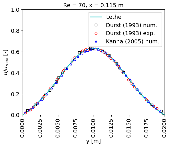
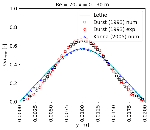
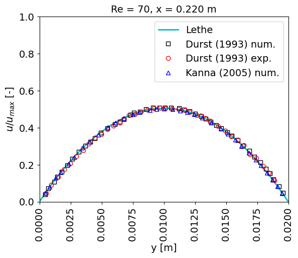
The first plot at \(x = 0.070\) m shows the Poiseuille-like flow before the channel expansion. A visible difference in the curves is noticed at \(x = 0.130\) m. Nonetheless, numerical results presented by Kanna et. al. [2] for this same example coincide with the Lethe curve.

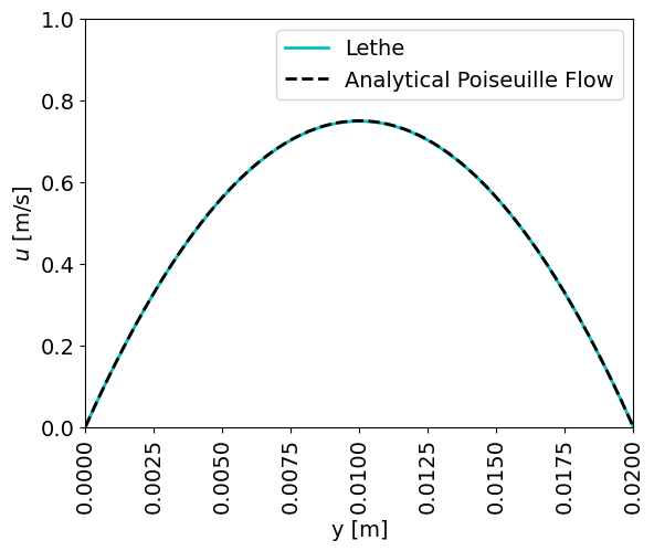
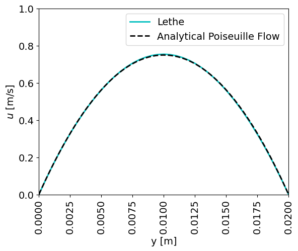
At \(x = L_{outlet}\) the velocity distribution is compared with analytical data, and a great agreement is found:

\(\mathrm{Re}=610\)

After running the simulation for \(\textrm{Re} = 610\), an asymmetric flow is observed at the final simulation time, where upper and lower recirculation zones at the beginning of \(L_{outlet}\) are uneven:

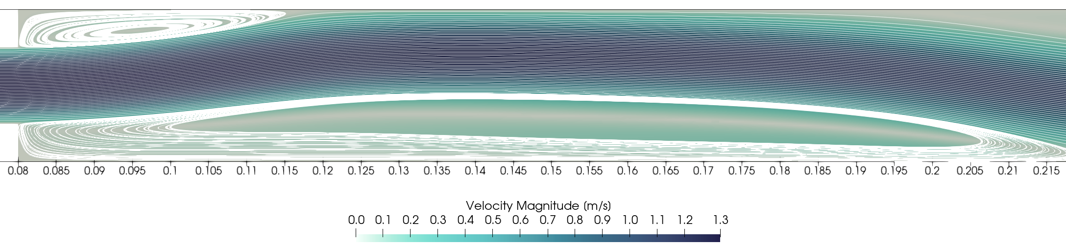
The velocity field variation over time is herein represented:

It is noticeable how oscillations happen at higher frequency after \(x \approx 0.25\) m; before that, the asymmetry in the outlet flow only becomes more pronounced after \(t \approx 2.5\) s. In this region, there is little change in the flow pattern after \(t \approx 4\) s.

The velocity profiles at different cross-sections can be visualized using the following command:

python3 velocity_profiles.py -Re 610

Comparing the velocity at the final simulation time with the results presented in Durst. et. al. [1] yields some discrepancies for \(x < 0.3\) m; nonetheless, curves have better agreement closer to the outlet:

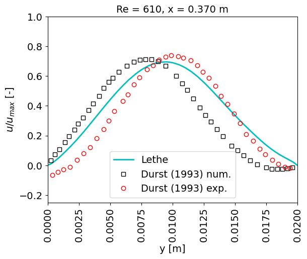
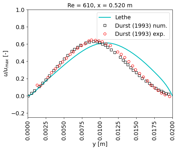
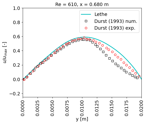
The discrepancies could be related to a number of factors, e.g. level of mesh discretization, adaptation algorithm, time step size, and type and parameters for the solver.

Similarly to the low-Reynolds number case, the outlet velocity profile is compared to the analytical Poiseuille flow solution, and a great agreement is obtained:

Possibilities for Extension

• Run the simulation with different Reynolds numbers: the sudden-expansion flow allows symmetric flow only up to a certain value of \(\textrm{Re}\), after which a bifurcation happens and asymmetric detachment appears. It can be interesting to change \(\textrm{Re}\) values to find the symmetric/asymmetric flow range.

• Alter mesh and solver parameters for the high Reynolds number case: as previously mentioned, the turbulent flow patterns might differ, for instance, when using a smaller time step, or a higher number of cells.

• Simulate a three-dimensional case: asymmetric effects can be even more pronounced once a three-dimensional flow is simulated and cross-sectional effects are taken into account.

References

[1] (1,2,3,4)

F. Durst, J. C. F. Pereira, C. Tropea. “The plane symmetric sudden-expansion flow at low Reynolds numbers”, J. Fluid Mech., vol. 248, pp. 567-581, Mar. 1993, doi: 10.1017/S0022112093000916.

[2]

P. Kanna, M. K. Das. “Numerical simulation of two-dimensional laminar incompressible offset jet flows”, Int. J. Numer. Meth. Fluids, vol. 49, no. 4, pp. 439-464, Oct. 2005, doi: 10.1002/fld.1007.