Transient Flow around an Ahmed Body

Features

• Solver: lethe-fluid (with Q1-Q1)

• Transient problem

• Displays how to import and easily adapt a gmsh file

• Displays how to run case in parallel with mpirun

Files Used in This Example

All files mentioned below are located in the example’s folder (examples/incompressible-flow/2d-ahmed-body).

• Geometry file: Ahmed-Body-20-2D.geo

• Mesh file: Ahmed-Body-20-2D.msh

• Parameter file: ahmed.prm

Description of the Case

In this example, a flow is passing across a fixed Ahmed body (simplified version of a car, classical benchmark for aerodynamic simulation tools). The velocity profile of the flow is simulated. The parameter file used is ahmed.prm.

The following schematic describes the simulation.

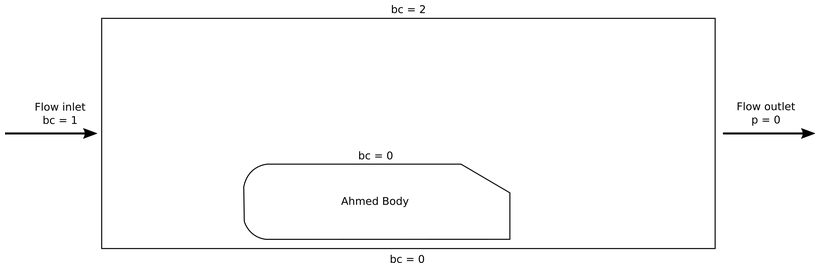
• bc = 0 (No slip boundary condition)

• bc = 1 (u = 1; flow in the x-direction)

• bc = 2 (Slip boundary condition)

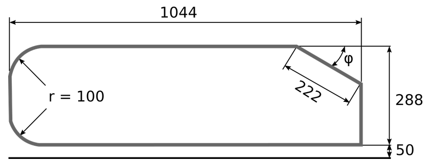
The basic geometry for the Ahmed body is given below, as defined in Ahmed et al. [1], with all measures in mm.

Parameter File

First, we import the mesh as in the 2D Flow around a cylinder.

Mesh

Geometry parameters can be adapted in the “Parameters” section of the .geo file, as shown below. Namely the step parameter phi can be easily adapted.

//===========================================================================
//Parameters
//===========================================================================
unit = 1000; //length unit : 1 -> mm ; 1000 -> m
phi = 20; //angle at rear, variable
esf = 2.0e-1; //element size factor, used in the free quad mesh

//Ahmed body basic geometry
L = 1044/unit;
H = 288/unit;
R = 100/unit;
Hw = 50/unit; //wheel height (height from the road)
Ls = 222/unit; //slope length

//Fluid domain
xmin = -500/unit;
ymin = -Hw;
xmax = 2500/unit;
ymax = 1000/unit;

The initial Mesh is built with Gmsh. It is defined as transfinite at the body boundary layer and between the body and the road, and free for the rest of the domain. The mesh is dynamically refined throughout the simulation. This will be explained later in this example.

The input mesh Ahmed-Body-20-2D.msh is in the same folder as the .prm file. The mesh subsection is set to use this file.

subsection mesh
  set type      = gmsh
  set file name = Ahmed-Body-20-2D.msh
end

Note

For further information about Mesh generation, we refer to the reader to the Introduction on How to Use GMSH page of this documentation, or the GridGenerator on the deal.ii documentation and the Gmsh website.

Initial and Boundary Conditions

The Initial Condition and Boundary Conditions are defined as in Example 3.

subsection initial conditions
  set type = nodal
  subsection uvwp
    set Function expression = 1; 0; 0
  end
end

subsection boundary conditions
  set number = 3
  subsection bc 0
    set type = noslip
  end
  subsection bc 1
    set type = function
    subsection u
      set Function expression = 1
    end
    subsection v
      set Function expression = 0
    end
    subsection w
      set Function expression = 0
    end
  end
  subsection bc 2
    set type = slip
  end
end

Simulation Control

Time integration is defined by a 1st order backward differentiation (bdf1), for a 4 seconds simulation (time end) with a 0.01 second time step. The output path is defined to save obtained results in a sub-directory, as stated in Simulation Control:

subsection simulation control
  set method           = bdf1
  set output frequency = 1
  set output name      = ahmed-output
  set output path      = ./Re720/
  set time end         = 4
  set time step        = 0.01
end

Warning

To successfully launch the simulation, the output path where the results are saved (in this example, the folder Re720) must already exist. Otherwise, the simulation will hang because it will be unable to save the results.

Ahmed bodies are typically studied considering a 60 m/s flow of air. Here, the flow speed is set to 1 (u = 1) so that the Reynolds number for the simulation (Re = uL/ν, with L the height of the Ahmed body) is varied by changing the kinematic viscosity:

subsection physical properties
  subsection fluid 0
    set kinematic viscosity = 4e-4
  end
end

Running the Simulation

The simulation is launched in the same folder as the .prm and .msh file, using the lethe-fluid solver. To decrease simulation time, it is advised to run on multiple cpu, using mpirun:

To do so, copy and paste the lethe-fluid executable to the same folder as your .prm file and launch it running the following line:

mpirun -np 6 lethe-fluid ahmed.prm

where 6 is the number of CPUs used. The estimated execution time for a 4 seconds simulation with 6 CPUs is 6 minutes and 53 seconds. For 1 CPU, the estimated time is 30 minutes and 37 seconds.

Alternatively, specify the path to the lethe-fluid in your build/applications folder, as follows:

mpirun -np 6 ../build/applications/lethe-fluid/lethe-fluid ahmed.prm

Guidelines for parameters other than the previous mentioned are found at the Parameters guide.

Results

Transient results are shown for three Re values:

Re	\({\nu}\)	Video	t = 0.5 s	t = 4 s
28.8	1e-2
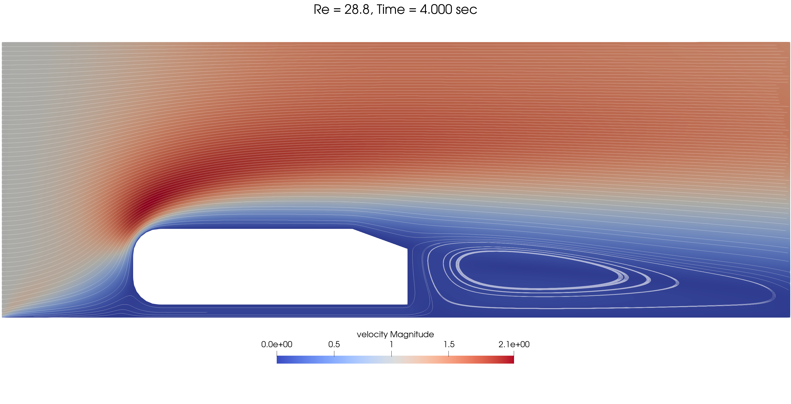
288	1e-3
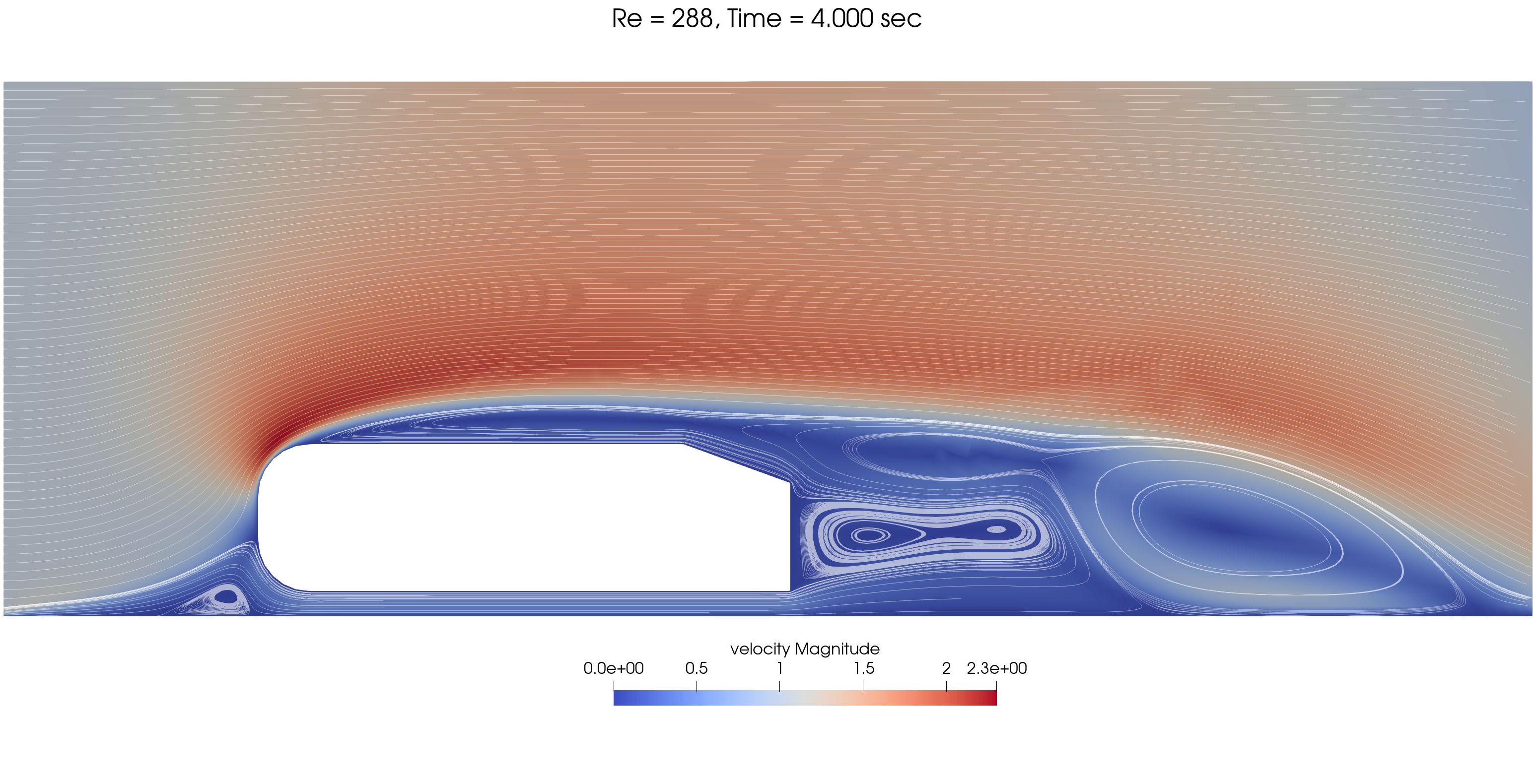
720	4e-2

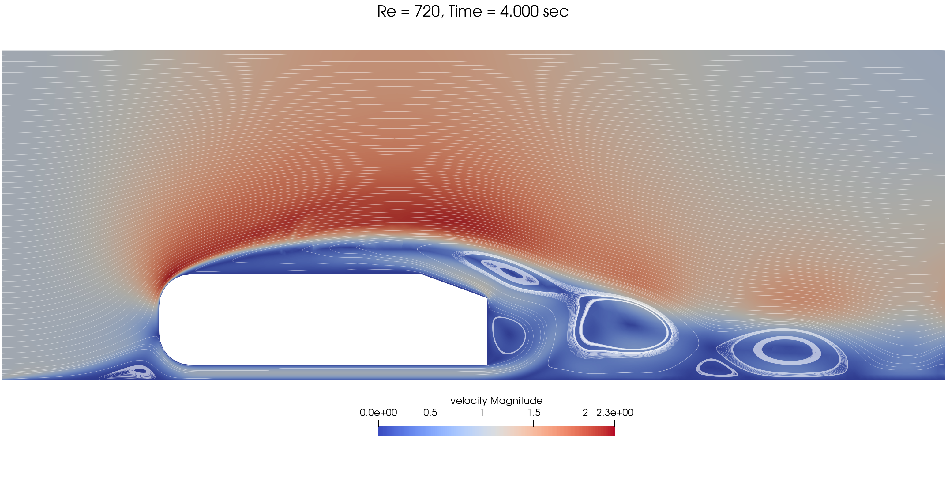
The mesh and processors load is adapted dynamically throughout the simulation, as shown below for Re = 720.

Time	Image
t = 0 s
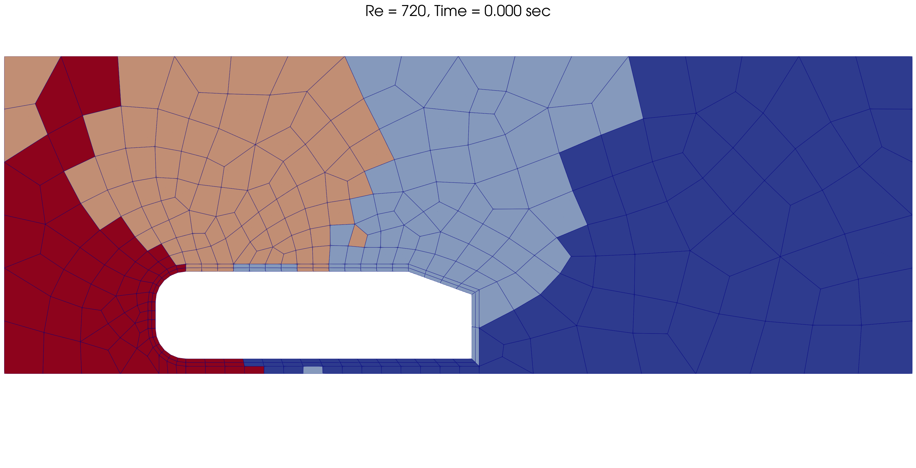
t = 0.05 s
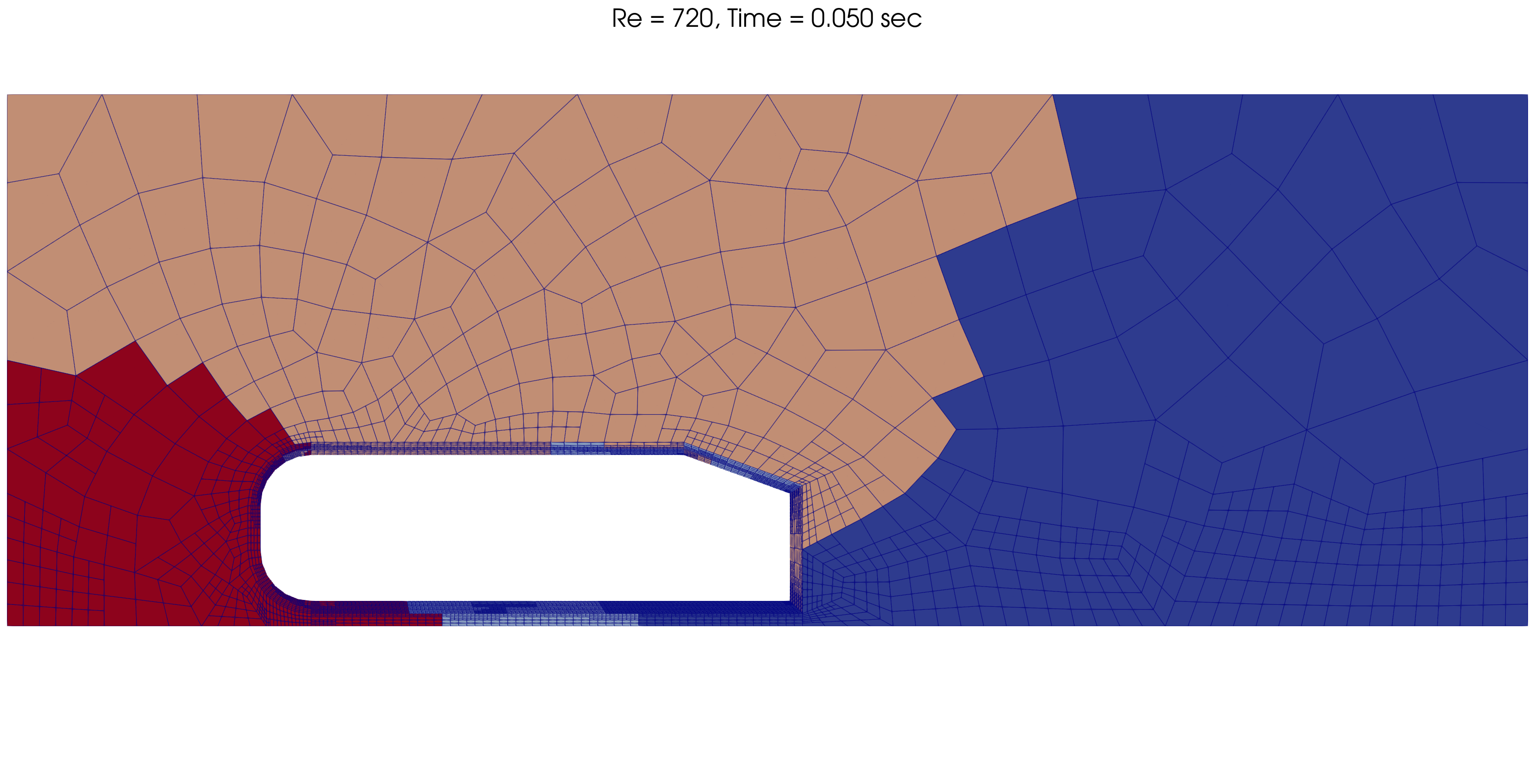
t = 4 s

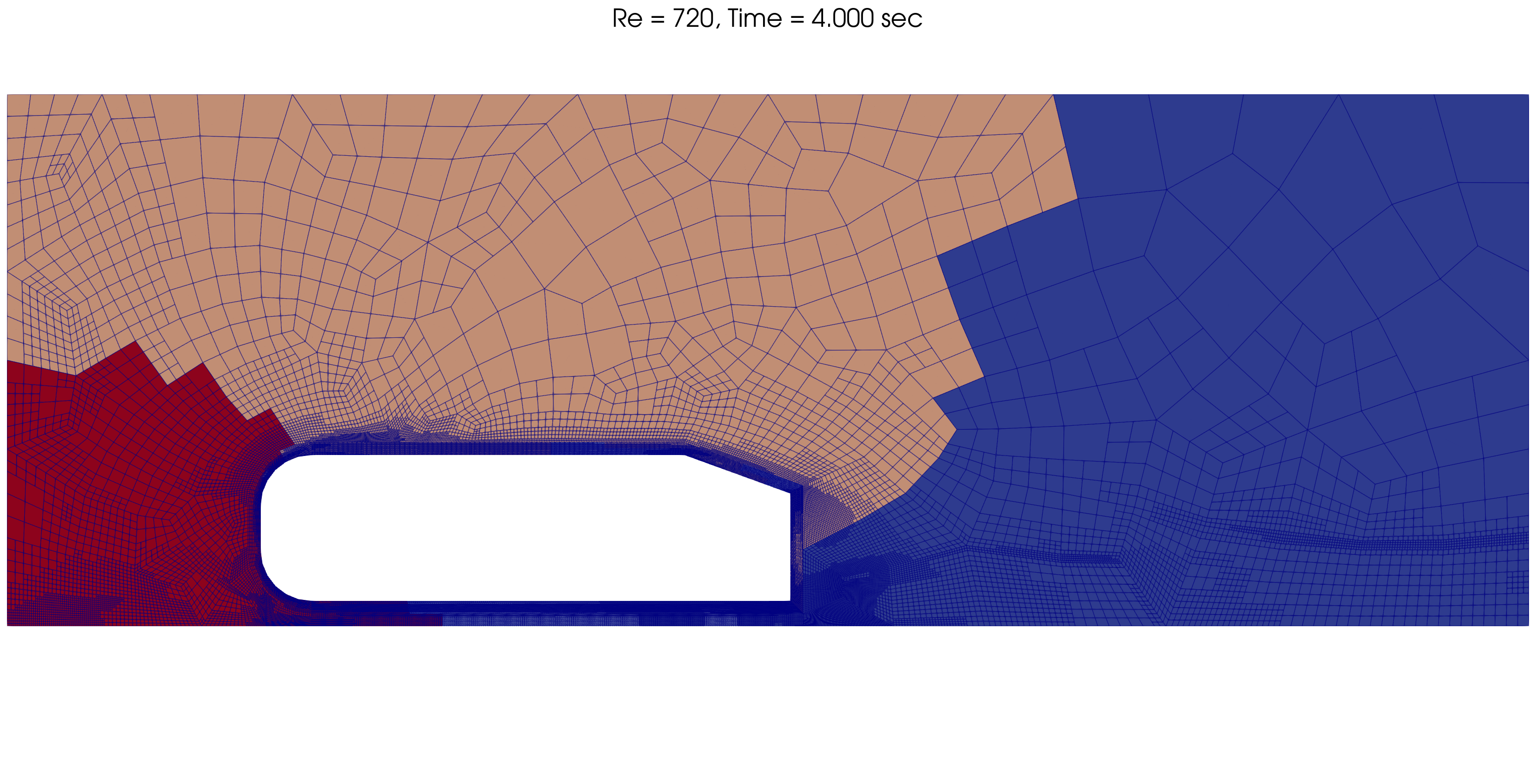
Possibilities for Extension

• Change the phi value to see the effect of the angle in the streamline.

• Vary the Reynolds number, or the initial and boundary conditions.

• Make a three-dimensional mesh, or even add other features to it, such as sharpen the edges.

• Test higher order elements (e.g., Q2-Q1).

Reference

[1]

Ahmed, S. R., et al. “Some Salient Features of the Time -Averaged Ground Vehicle Wake.” SAE Transactions, vol. 93, pp. 473–503, 1984. http://www.jstor.org/stable/44434262.