Flow around a Cylinder Using the Sharp Interface Method#
Features#
Solvers:
lethe-fluid-sharp(with Q1-Q1)Steady-state problem
Explains how to set sharp interface immersed boundary to represent a particle
Displays the use of non-uniform mesh adaptation
Files Used in this Example#
Parameter file:
examples/sharp-immersed-boundary/cylinder-with-sharp-interface/cylinder-with-sharp-interface.prm
Description of the Case#
Mesh#
In this example, we study the flow around a static cylinder in 2D using the sharp-interface method to represent the cylinder. The geometry of the flow takes the same basic case defined in Flow around a Cylinder. As such, we use the parameter file associated with Flow around a Cylinder as the base for this example. The exact dimensions for this example can be found in the following figure.
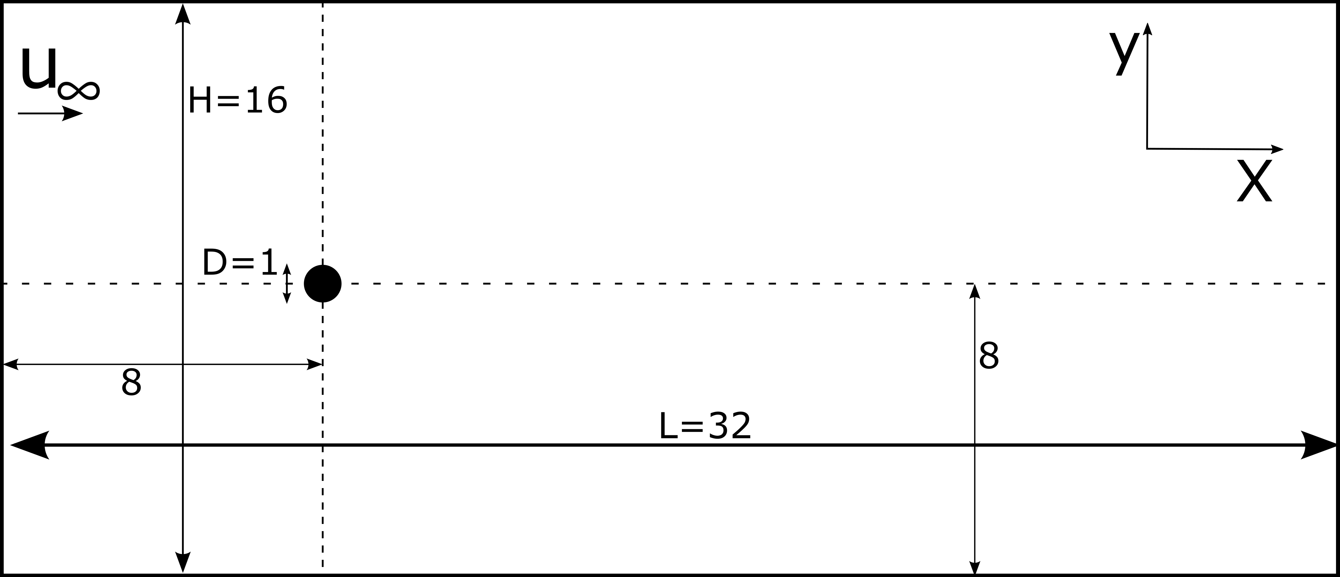
This case uses a cartesian structured rectangular mesh, and we define the position and radius of the immersed cylinder.
The mesh is defined using the following subsection.
subsection mesh
    set type               = dealii
    set grid type          = subdivided_hyper_rectangle
    set grid arguments     = 2,1: 0,0 : 32 , 16  : true
    set initial refinement = 7
end
Boundary Conditions#
As for the Flow around a Cylinder, we define the boundary conditions to have an inlet on the left, two slip boundary conditions at the top and bottom, and an outlet on the right of the domain.
subsection boundary conditions
  set number = 4
  subsection bc 0
    set id   = 0
    set type = function
    subsection u
      set Function expression = 1
    end
    subsection v
      set Function expression = 0
    end
    subsection w
      set Function expression = 0
    end
  end
  subsection bc 1
    set id   = 1
    set type = outlet
  end
  subsection bc 2
    set id   = 2
    set type = slip
  end
  subsection bc 3
    set id   = 3
    set type = slip
  end
end
Initial Conditions#
The initial condition has been modified compared to the initial solution proposed in Flow around a Cylinder. We use the following initial condition to ensure that the particle’s boundary condition is satisfied.
subsection initial conditions
  set type = nodal
  subsection uvwp
    set Function expression = 0; 0; 0
  end
end
IB Particles#
The only thing that is left to define is the immersed boundary. In this case, we want to define a circular boundary of radius 0.5 centered at (8,8) that has no velocity. We use the sphere to model the cylinder in 2D.
subsection particles
  set number of particles                     = 1
  subsection extrapolation function
    set stencil degree = 2
  end
  subsection local mesh refinement
    set initial refinement                = 0
  end
  subsection particle info 0
    set type             = sphere
    set shape arguments  = 0.5
    subsection position
      set Function expression = 8;8
    end
    subsection velocity
      set Function expression = 0;0
    end
  end
end
number of particlesis set to1as we only want one particle.stencil degreeis set to2as this is the highest degree that is compatible with the FEM scheme and it does not lead to Runge instability. The highest degree of stencil compatible with a FEM scheme is defined by the polynomial degree of the scheme time the number of dimensions: in this case, 2.initial refinementis set to 0. In this case, the initial mesh is small enough compared to the particle size. It is therefore not necessary to pre-refine the mesh around the particle.positionFunction expression is set to8;8as the position of the particle is constant in time.velocityFunction expression is set to0;0as this is a steady and static case.
All the other parameters have been set to their default values since they do not play a role in this case.
Results#
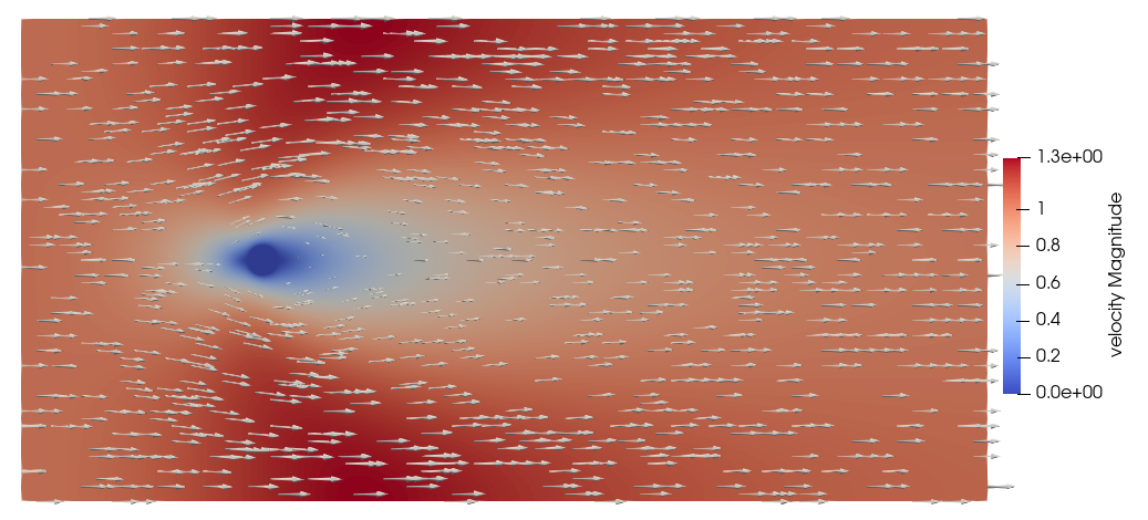
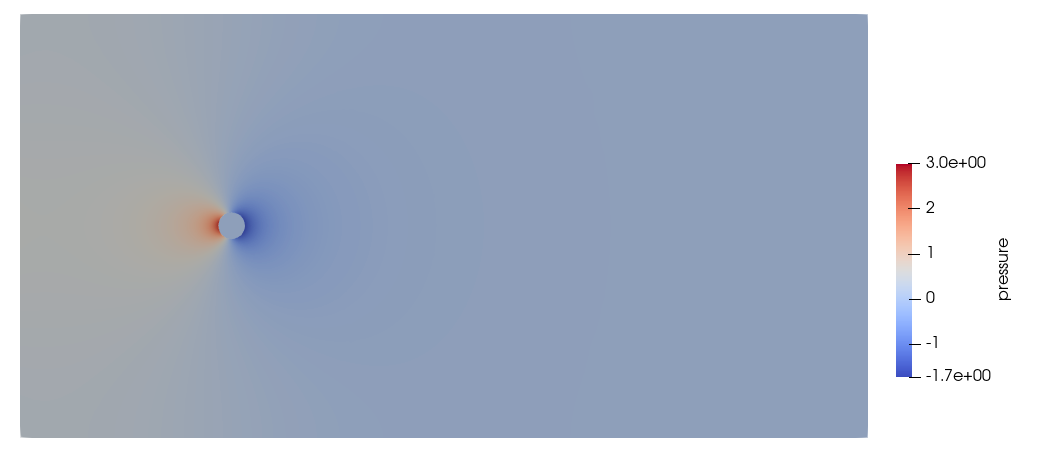
The simulation of this case results in the following solution for the velocity and pressure field.
Velocity:
Pressure:
We get the following force applied to the particle for each of the mesh refinements, which is similar to the one obtained with a conformal mesh in Flow around a Cylinder. With the conformal mesh, the drag force applied to the particle is \(7.123\). The difference between the results from using a conformal or a non-conformal mesh can be attributed to the discretization error.
particle_ID    T_z        f_x         f_y
        0   -0.006703   6.447400    0.004273
        0   -0.000389   6.775330    0.000379
        0   -0.000040   6.906123    0.000377
        0   -0.000053   6.962566    0.000310
        0   -0.000039   6.992112    0.000193
Note
The drag coefficient obtained in this case is higher than the drag coefficient for a cylinder at a Reynolds number of 1 as the size of the domain is not large enough relative to the diameter of the cylinder. The flow around the cylinder is then constrained by the lateral boundaries, and this increases the drag coefficient.