Transient Flow around a Cylinder

This example corresponds to a transient flow around a fixed cylinder at a high Reynolds number.

Features

• Solver: lethe-fluid (with Q2-Q1)

• Transient problem

• Usage of Gnuplot and Python scripts for the data post-processing

Files Used in This Example

All files mentioned below are located in the example’s folder (examples/incompressible-flow/2d-transient-flow-around-cylinder).

• Geometry file: cylinder-structured.geo

• Mesh file: cylinder-structured.msh

• Parameter file: cylinder.prm

Description of the Case

We simulate the flow around a fixed cylinder with a constant upstream fluid velocity. We re-use the geometry and mesh presented in 2D Flow around a cylinder, which were taken from Blais et al. [1]:

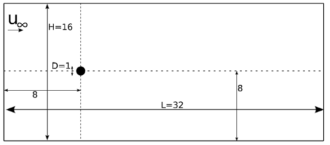
The flow field features a stable laminar boundary layer at the cylinder leading edge and a recirculation zone behind it formed by two unstable vortices of opposite signs. These vortices successively detach from the cylinder in a periodic manner (vortex shedding), leading to the generation of the von Kármán vortex street pattern in the wake. This vortex shedding causes a fluctuating pressure force acting on the cylinder, resulting in oscillations of the drag and lift coefficients in time. The frequency of vortex shedding is related to the Strouhal number:

\[S_t = \frac{D f_v}{U_\infty}\]

where \(D\) is the diameter of the cylinder, \(f_v\) is the frequency of the shedding and \(U_\infty\) is the upstream velocity.

Parameter File

Simulation Control

This example uses a 2nd order backward differentiation (method = bdf2) for the time integration scheme. The simulation time is set to 200 seconds with the time end parameter and a time step of 0.05 seconds is used (time step = 0.05).

subsection simulation control
  set method           = bdf2
  set output name      = cylinder-output
  set output frequency = 5
  set output path      = ./Re200/
  set time end         = 200.0
  set time step        = 0.05
end

FEM Interpolation

The interpolation orders for the velocity and pressure are set to Q2-Q1 in the FEM subsection:

subsection FEM
  set velocity order = 2
  set pressure order = 1
end

Mesh

The initial mesh is generated with Gmsh and imported as described in 2D Flow around a cylinder.

subsection mesh
  set type               = gmsh
  set file name          = cylinder-structured.msh
  set initial refinement = 1
end

Mesh Adaptation

While the discretization in the wake of the cylinder has less impact on the forces acting on the cylinder wall than the boundary layer discretization, it is interesting to well resolve the wake to capture the von Kármán vortex street pattern. Therefore, to adapt the mesh in the boundary layer and the wake as the vortices are shed, a non-uniform mesh adaptation is performed at each time step and the parameters are specified using the Mesh Adaptation subsection:

subsection mesh adaptation
  set type                 = kelly
  set variable             = pressure
  set fraction type        = number
  set max number elements  = 70000
  set max refinement level = 3
  set min refinement level = 1
  set frequency            = 1
  set fraction refinement  = 0.02
  set fraction coarsening  = 0.01
end

Here, we are using the pressure as the variable for the Kelly error estimator, unlike the previous examples which were using the velocity. Indeed, we have observed that the refinement has less tendency to follow the vortices as they move through the wake with the pressure as the refinement indicator than if we select the velocity. Additionally, the fraction refinement and fraction coarsening are set to lower values than the previous examples (i.e., respectively 0.02 and 0.01) to enable a gradual growth of the mesh size.

Initial and Boundary Conditions

The Initial Condition and Boundary Conditions are defined as in 2D Flow around a cylinder.

subsection initial conditions
  set type = nodal
  subsection uvwp
    set Function expression = 1; 0; 0
  end
end

subsection boundary conditions
  set number = 3
  subsection bc 0
    set type = noslip
  end
  subsection bc 1
    set type = function
    subsection u
      set Function expression = 1
    end
    subsection v
      set Function expression = 0
    end
    subsection w
      set Function expression = 0
    end
  end
  subsection bc 2
    set type = slip
  end
end

Physical Properties

The Reynolds number must be high enough to capture a transient flow and study the evolution of the drag and lift coefficients in time. Therefore, we set Re = 200 through the value of the kinematic viscosity in the same manner as for the 2D Lid-driven cavity flow. Since \(U_\infty = 1\) and the \(D = 1\), we have \(Re=\frac{1}{\nu}\), where \(\nu\) is the kinematic viscosity.

subsection physical properties
  subsection fluid 0
    set kinematic viscosity = 0.005
  end
end

Linear Solver

For 2D problems, the amg preconditioner is an adequate preconditioner. It is especially robust for the first few time-steps for which the velocity and pressure profile is not well-defined because the initial conditions are not mass conservative.

subsection linear solver
  subsection fluid dynamics
    set verbosity                                 = verbose
    set method                                    = gmres
    set relative residual                         = 1e-4
    set minimum residual                          = 1e-8
    set preconditioner                            = amg
    set amg preconditioner ilu fill               = 0
    set amg preconditioner ilu absolute tolerance = 1e-12
    set amg preconditioner ilu relative tolerance = 1.00
  end
end

Forces

Since we want to study the time evolution of the drag and lift coefficients, the force acting on the boundaries must be computed. We thus use the forces subsection:

subsection forces
  set verbosity             = verbose
  set calculate force       = true
  set calculate torque      = false
  set force name            = force
  set output precision      = 10
  set calculation frequency = 1
  set output frequency      = 10
end

As we set calculation frequency to 1, the forces on each boundary are computed at each time step and written in the file specified by the field force name.

Note

The drag and lift coefficients are obtained with the forces acting on the wall of the cylinder (i.e., f_x and f_y written in the file forces.00.dat) :

\[C_D = \frac{2 f_x}{\rho U_\infty^2 D} \text{ and } C_L = \frac{2 f_y}{\rho U_\infty^2 D}\]

where \(\rho = 1\). This way, we can obtain the evolution in time of both coefficients.

Warning

The computational cost of writing this output file at each time step by setting output frequency to 1 can be significant, as explained in Force and torque calculation. It is a good practice to set output frequency to higher values, such as 10-100, to reduce the computational cost.

Running the Simulation

The simulation is launched in parallel using 10 CPUs, as explained in 2D Transient flow around an Ahmed body :

mpirun -np 10 lethe-fluid cylinder.prm

Warning

The estimated time to simulate 200 seconds is about 3 hours with 10 CPUs.

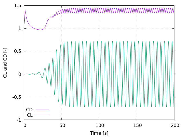
Results

The time evolution of the drag and lift coefficients is obtained from a Gnuplot script available in the example folder by launching in the same directory the following command:

gnuplot -c "./postprocess.gnu" "./Re200"

where ./postprocess.gnu is the path to the provided script and ./Re200 is the path to the directory that contains the simulation results (specified in the simulation control subsection). The figure, named CL-CD.png, is outputted in the directory ./Re200.

Note

Gnuplot is a command-line plotting tool supporting scripting. It can be downloaded here. The script provided for this example works for the version 5.4 of Gnuplot.

Using the fast Fourier transform (FFT) of the CL for the last 100 seconds, we can obtain the frequency \(f_v\) at which the vortices are shed :

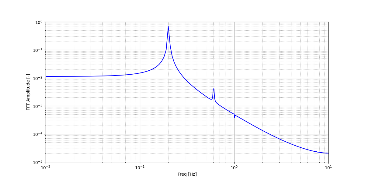
This corresponds to the frequency at which the peak of amplitude appears in the FFT : \(f_v = 0.2\). From this result, we can obtain the Strouhal number, \(S_t = 0.2\), using the equation presented above. The python script used to obtain the FFT is available in the example folder and is launched in the same directory using the following command:

python ./postprocess.py ./Re200

where ./postprocess.py is the path to the provided script and ./Re200 is the path to the directory that contains the simulation results (specified in the simulation control subsection). The figure, named cylinderFFT.png, is outputted in the directory ./Re200.

The obtained values of the drag and lift coefficients as well as the Strouhal number are compared to some results of the literature :

Study	\(C_D\)	\(C_L\)	\(S_t\)
Lethe example	1.396 \(\pm\) 0.048	-0.003 \(\pm\) 0.072	0.2
Lethe Sharp [2]	1.395 \(\pm\) 0.047	\(\pm\) 0.071	0.2
Braza et al. [3]	1.400 \(\pm\) 0.050	\(\pm\) 0.075	0.2

Using Paraview the following velocity and pressure fields can be visualized in time:

Possibilities for Extension

• Study the vortex shedding of other bluff bodies.

• Increase the Reynolds number to study a completely turbulent wake and the drag crisis phenomenon.

• Repeat the same example in 3D for a cylinder/sphere and study the effect on the drag and lift forces.

• Investigate the impact of the time-step and the time-stepping scheme (e.g., bdf 3)

References

[1]

B. Blais, M. Lassaigne, C. Goniva, L. Fradette, and F. Bertrand, “A semi-implicit immersed boundary method and its application to viscous mixing,” Comput. Chem. Eng., vol. 85, pp. 136–146, Feb. 2016, doi: 10.1016/j.compchemeng.2015.10.019.

[2]

L. Barbeau, S. Étienne, C. Béguin, and B. Blais, “Development of a high-order continuous Galerkin sharp-interface immersed boundary method and its application to incompressible flow problems,” Comput. Fluids, vol. 239, p. 105415, May 2022, doi: 10.1016/j.compfluid.2022.105415.

[3]

M. Braza, P. Chassaing, and H. H. Minh, “Numerical study and physical analysis of the pressure and velocity fields in the near wake of a circular cylinder,” J. Fluid Mech., vol. 165, pp. 79–130, Apr. 1986, doi: 10.1017/S0022112086003014.