Physical Properties

Note

Lethe supports single phase, two phase (using VOF) and conjugate simulations. This is managed using the fluid and solid subsections.

subsection physical properties
  set number of fluids      = 1
  set reference temperature = 0
  subsection fluid 0
    # Rheology
    set rheological model          = newtonian
    set kinematic viscosity        = 1

    # Density
    set density model              = constant
    set density                    = 1

    # Specific heat
    set specific heat model        = constant
    set specific heat              = 1

    # Thermal conductivity
    set thermal conductivity model = constant
    set thermal conductivity       = 1

    # Thermal expansion
    set thermal expansion model    = constant
    set thermal expansion          = 0

    # Tracer diffusivity
    set tracer diffusivity model   = constant
    set tracer diffusivity         = 0
  end

  set number of solids = 0

  set number of material interactions = 1 #by default it is set to 0
  subsection material interaction 0
    set type = fluid-fluid
    subsection fluid-fluid interaction
      set first fluid id              = 0
      set second fluid id             = 1

      # Surface tension
      set surface tension model                       = constant
      set surface tension coefficient                 = 0
      set reference state temperature                 = 0
      set temperature-driven surface tension gradient = 0
      set liquidus temperature                        = 0
      set solidus temperature                         = 0

      # Mobility Cahn-Hilliard
      set cahn hilliard mobility model    = constant
      set cahn hilliard mobility constant = 1e-7
    end

    # if fluid-solid interaction
    subsection fluid-solid interaction
      set fluid id                    = 0
      set solid id                    = 0

      # Surface tension
      set surface tension model                       = constant
      set surface tension coefficient                 = 0
      set reference state temperature                 = 0
      set temperature-driven surface tension gradient = 0
      set liquidus temperature                        = 0
      set solidus temperature                         = 0
    end
  end
end

• The number of fluids parameter controls the number of fluids in the simulation. This parameter is set to 1 except in Two Phase Simulations .

• The reference temperature parameter specifies the reference temperature used in the calculation of some physical properties or the thermal expansion force.

  • The rheological model parameter sets the choice of rheological model. The choices are between newtonian, power-law, carreau and phase_change. For more details on the rheological models, see Rheological Models .

  • The kinematic viscosity parameter is the kinematic viscosity of the newtonian fluid in units of \(\text{Length}^{2} \cdot \text{Time}^{-1}\). In SI, this is \(\text{m}^{2} \cdot \text{s}^{-1}\). This viscosity is only used when rheological model = newtonian.

  • The density model specifies the model used to calculate the density. At the moment, a constant density and an isothermal_ideal_gas model are supported. For more details on the density models, see Density Models.

  • The density parameter is the constant density of the fluid in units of \(\text{Mass} \cdot \text{Length}^{-3}\)

  • The specific heat model specifies the model used to calculate the specific heat. At the moment, only a constant specific heat is supported.

  • The specific heat parameter is the constant specific heat of the fluid in units of \(\text{Energy} \cdot \text{Temperature}^{-1} \cdot \text{Mass}^{-1}\) .

  • The thermal conductivity model specifies the model used to calculate the thermal conductivity. At the moment, constant and linear thermal conductivity are available. For more details on the thermal conductivity models, see Thermal Conductivity Models.

  • The thermal conductivity parameter is the thermal conductivity coefficient of the fluid with units of \(\text{Power} \cdot \text{Temperature}^{-1} \cdot \text{Length}^{-1}\).

  • The thermal expansion model specifies the model used to calculate the thermal expansion coefficient. At the moment, constant and phase_change thermal expansion are supported. For more details on the thermal expansion models, see Thermal Expansion Models.

  • The thermal expansion parameter is the thermal expansion coefficient of the fluid with dimension of \(\text{Temperature}^{-1}\). It is used to define the buoyancy-driven flow (natural convection) using the Boussinesq approximation, which leads to the definition of the following source term that is added to the Navier-Stokes equation:

    \[{\bf{F_{B}}} = -\beta {\bf{g}} (T-T_\text{ref})\]

    where \(F_B\) denotes the buoyant force source term, \(\beta\) is the thermal expansion coefficient, \(T\) is temperature, and \(T_\text{ref}\) is the reference temperature. This is only used when a constant thermal expansion model is used.

  • The tracer diffusivity model specifies the model used to calculate the tracer diffusivity. At the moment, a constant tracer diffusivity and level set based \(\tanh\) model are supported. The immersed solid tanh model is intended to be used with immersed solids with the lethe-fluid-sharp executable as a way to set diffusivity inside solids as well (described more in Immersed Solid Models).

  • The tracer diffusivity parameter is the diffusivity coefficient of the tracer in units of \(\text{Length}^{2} \cdot \text{Time}^{-1}\) . In SI, this is \(\text{m}^{2} \cdot \text{s}^{-1}\).

• The number of solids parameter controls the number of solid regions. Solid regions are currently only implemented for Conjugate Heat Transfer.

• The number of material interactions parameter controls the number of physical properties that are due to the interaction between two materials. At the moment, only the surface tension between two fluids is implemented in Two Phase Simulations.

  • The material interaction type can either be fluid-fluid (default) or fluid-solid.

  • In the fluid-fluid subsection we define the pair of fluids and their physical properties.

    • The first fluid id is the id of the first fluid.

    • The second fluid id is the id of the second fluid.

      Attention

      The second fluid id should be greater than the first fluid id.

    • The surface tension model specifies the model used to calculate the surface tension coefficient of the fluid-fluid pair. At the moment, constant, linear, and phase_change models are supported. For more details on the surface tension models, see Surface Tension Models.

    • The surface tension coefficient parameter is a constant surface tension coefficient of the two interacting fluids in units of \(\text{Mass} \cdot \text{Time}^{-2}\). In SI, this is \(\text{N} \cdot \text{m}^{-1}\). The surface tension coefficient is used as defined in the Weber number (\(We\)):

      \[We = Re \cdot \frac{\mu_\text{ref} \; u_\text{ref}}{\sigma}\]

      where \(Re\) is the Reynolds number, \(\mu_\text{ref}\) and \(u_\text{ref}\) are some reference viscosity and velocity characterizing the flow problem, and \(\sigma\) is the surface tension coefficient.

    • The reference state temperature parameter is the temperature of the reference state at which the surface tension coefficient is evaluated. This parameter is used in the calculation of the surface tension using the linear surface tension model (see Surface Tension Models).

    • The temperature-driven surface tension gradient parameter is the surface tension gradient with respect to the temperature of the two interacting fluids in units of \(\text{Mass} \cdot \text{Time}^{-2} \cdot \text{Temperature}^{-1}\). In SI, this is \(\text{N} \cdot \text{m}^{-1} \cdot \text{K}^{-1}\). This parameter is used in the calculation of the surface tension using the linear surface tension model (see Surface Tension Models).

    • The solidus temperature and liquidus temperature parameters are used in the calculation of the surface tension using the phase_change surface tension model (see Surface Tension Models).

    • The cahn hilliard mobility model specifies the model used to calculate the mobility used in the Cahn-Hilliard equations for the pair of fluid. Two models are available: a constant mobility and a quartic mobility. The reader is refered to Cahn-Hilliard for more details.

    • The cahn hilliard mobility coefficient parameter is the constant mobility coefficient of the two interacting fluids used in the Cahn-Hilliard equations. Its units are \(\text{Length}^{2} \cdot \text{Time}^{-1}\).

  • In the fluid-solid subsection we define the fluid-solid pair and their physical properties.

    • The fluid id is the id of the fluid.

    • The solid id is the id of the solid.

    • The surface tension model and surface tension coefficient are the same as described in the fluid-fluid subsection above.

Note

The default values for all physical properties models in Lethe is constant. Consequently, it is not necessary (and not recommended) to specify the physical property model unless this model is not constant. This generates parameter files that are easier to read.

Material Physical Property Models

Two Phase Simulations

Note

Two phase simulations require that either set VOF = true or set cahn hilliard = true in the Multiphysics subsection. By convention, air is usually the fluid 0 and the other fluid of interest is the fluid 1.

For two phases, the properties are defined for each fluid. Default values are:

subsection physical properties
set number of fluids = 2
    subsection fluid 0
       set density              = 1
       set kinematic viscosity  = 1
       set specific heat        = 1
       set thermal conductivity = 1
       set tracer diffusivity   = 0
    end
    subsection fluid 1
       set density              = 1
       set kinematic viscosity  = 1
       set specific heat        = 1
       set thermal conductivity = 1
       set tracer diffusivity   = 0
    end
end

• number of fluids = 2 is required for a free surface simulation, otherwise an error will be thrown in the terminal.

• subsection fluid 0 indicates the properties of fluid where the phase indicator = 0 (Volume of Fluid method), as defined when initializing the free surface (see the Initial Conditions subsection), and correspondingly fluid 1 is located where the phase indicator = 1.

Warning

Lethe now supports the use of physical properties models that are different for both phases. For example, the liquid could have a carreau rheological model and the air could have a newtonian rheological model. However, this feature has not been fully tested and could lead to unpredictable results. Use with caution.

Conjugate Heat Transfer

Conjugate heat transfer enables the addition of solid regions in which the fluid dynamics is not solved for. To enable the presence of a solid region, number of solids must be set to 1. By default, the region with the material_id=0 will be the fluid region whereas the region with material_id=1 will be the solid region. The physical properties of the solid region are set in an identical fashion as those of the fluid.

Warning

This is an experimental feature. It has not been tested on a large range of application cases.

subsection physical properties
  set number of fluids = 1
  subsection fluid 0
    ...
  end
  set number of solids = 1
  subsection solid 0
    # Density
    set density model              = constant
    set density                    = 1

    # Specific heat
    set specific heat model        = constant
    set specific heat              = 1

    # Thermal conductivity
    set thermal conductivity model = constant
    set thermal conductivity       = 1
  end
end

Immersed Solid Models

Immersed solid models can be used to affect specific behavior to immersed solids when lethe-fluid-sharp is used. At the moment, such a model is only available for the tracer multiphysics, but additional physics will be included in the future.

The immersed solid properties models are based on the signed distance function of the immersed solids, and therefore depend on the depth inside the solid. The intent behind these models is to define physical properties in the fluid and solid phases as well as in the transition regions.

The tracer diffusivity model parameter sets which diffusivity model is used. The default model is constant, which uses a constant tracer diffusivity. The alternative is immersed solid tanh, whose parameters are defined as such, with \(D\) being the tracer diffusivity (outside and inside), \(\lambda\) being signed distance and \(t\) the thickness of the transition zone between both diffusivity values:

\[D(\lambda) = D_\text{inside} + \left(D_\text{outside} - D_\text{inside}\right) \left( 0.5 + 0.5 \tanh \left(\frac{\lambda}{t}\right)\right)\]

subsection physical properties
  set number of fluids = 1
  subsection fluid 0
    set kinematic viscosity = 0.01
    set tracer diffusivity model = immersed solid tanh
    subsection immersed solid tanh
      set tracer diffusivity inside    = 1
      set tracer diffusivity outside   = 1
      set thickness                    = 1
    end
  end
end

• The tracer diffusivity inside parameter represents the desired diffusivity inside of the solid.

• The tracer diffusivity outside parameter represents the desired diffusivity outside of the solid.

• The thickness parameter represents thickness of the applied \(\tanh\) function.

Rheological Models

Two families of rheological models are supported in Lethe. The first one are generalized non Newtonian rheologies (for shear thinning and shear thickening flows). In these models, the viscosity depends on the shear rate. The second family of rheological models possess a viscosity that is independent of the shear rate, but that may depend on other fields such as the temperature.

The rheological model parameter sets which rheological model you are using. The default rheological model is newtonian, which uses a constant kinematic viscosity.

subsection physical properties
  set number of fluids = 1
  subsection fluid 0
    set rheological model   = newtonian
    set kinematic viscosity = 1.0
  end
end

The rheological model available options are:

• newtonian

• power-law

• carreau

• phase_change

Power-Law Model

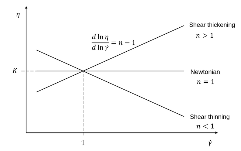
The power-law model is the simplest rheological model, using only 2 parameters

\[\eta(\dot{\gamma}) = K \dot{\gamma}^{n-1}\]

where \(\eta\) is the kinematic viscosity and \(\dot{\gamma}\) is the local shear rate magnitude.

When using the power-law model, the default values are:

subsection physical properties
  set number of fluids = 1
  subsection fluid 0
    set rheological model   = power-law
    subsection non newtonian
      subsection power-law
        set K               = 1.0
        set n               = 0.5
        set shear rate min  = 1e-3
      end
    end
  end
end

• The K parameter is a fluid consistency index. It represents the fluid viscosity for a local shear rate of \(1.0\).

• The n parameter is the flow behavior index. It sets the slope in the log-log \(\eta = f(\dot{\gamma})\) graph.

• The shear rate min parameter yields the magnitude of the shear rate tensor for which the viscosity is calculated. Since the model uses a power operation, a null shear rate magnitude leads to an invalid viscosity. To ensure numerical stability, the shear rate cannot go below this threshold when the viscosity calculated.

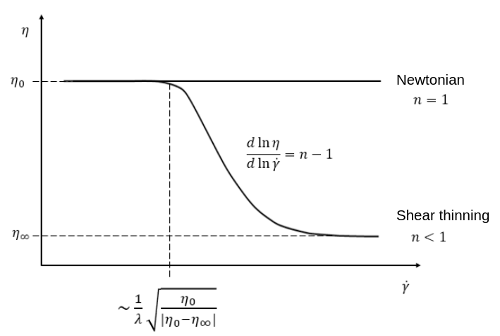
Carreau Model

The Carreau model is in reality the five parameter Carreau model:

\[\eta(\dot{\gamma}) =\eta_{\infty} + (\eta_0 - \eta_{\infty}) \left[ 1 + (\dot{\gamma}\lambda)^a\right]^{\frac{n-1}{a}}\]

where \(\eta\) is the kinematic viscosity and \(\dot{\gamma}\) is the shear rate.

The parameters for the Carreau model are defined by the carreau subsection. The default values are:

subsection physical properties
  set number of fluids = 1
  subsection fluid 0
    set rheological model   = carreau
    subsection non newtonian
      subsection carreau
        set viscosity_0     = 1.0
        set viscosity_inf   = 1.0
        set a               = 2.0
        set lambda          = 1.0
        set n               = 0.5
      end
    end
  end
end

• The viscosity_0 parameter represents the viscosity when the shear rate on the fluid tends to 0.

• The viscosity_inf parameter represents the viscosity when the shear rate on the fluid becomes large.

• The a is the Carreau parameter, generally set to 2.

• The lambda is the relaxation time associated to the fluid.

• The n is a power parameter. It sets the slope in the log-log \(\eta = f(\dot{\gamma})\) graph just like in the power-law model.

Note

The Carreau model is only suitable for Newtonian and shear-thinning flows.

Phase-Change Model

The phase change model is a simple rheological model in which the viscosity depends on the temperature. This model is used to model melting and freezing of components. The kinematic viscosity \(\nu\) is given by :

\[\begin{split}\nu = c^{*}_\text{p} = \begin{cases} \nu_\text{s} & \text{if} \; T<T_\text{s} \\ \frac{T-T_\text{s}}{T_\text{l}-T_\text{s}} \nu_\text{l} + \left(1-\frac{T-T_\text{s}}{T_\text{l}-T_\text{s}}\right) \nu_\text{s} & \text{if} \; T_\text{l}>T>T_\text{s}\\ \nu_\text{l} & \text{if} \; T>T_\text{l} \end{cases}\end{split}\]

where \(T_\text{l}\) and \(T_\text{s}\) are the liquidus and solidus temperature. The underlying hypothesis of this model is that the melting and the solidification occur over a phase change interval. Melting will occur between \(T_\text{s}\) and \(T_\text{l}\) and solidification will occur between \(T_\text{l}\) and \(T_\text{s}\).

This model is parameterized using the phase change subsection

subsection phase change
  # Temperature of the liquidus
  set liquidus temperature = 1

  # Temperature of the solidus
  set solidus temperature  = 0

  # Viscosity of the liquid phase
  set viscosity liquid     = 1

  # Viscosity of the solid phase
  set viscosity solid      = 1
end

• The liquidus temperature is \(T_\text{l}\)

• The solidus temperature is \(T_\text{s}\)

• The viscosity liquid is \(\nu_\text{l}\)

• The viscosity solid is \(\nu_\text{s}\)

Note

The phase change subsection is used to parametrize both rheological model = phase_change and specific heat model = phase_change. This prevents parameter duplication.

Density Models

Lethe supports both constant and isothermal_ideal_gas density models. Constant density assumes a constant density value. Isothermal ideal gas density assumes that the fluid’s density varies according the following state equation:

\[\rho = \rho_\text{ref} + \psi p = \rho_\text{ref} + \frac{1}{R T} \ p\]

where \(\rho_\text{ref}\) is the density of the fluid at the reference state, \(\psi = \frac{1}{R T}\) is the compressibility factor derived from the ideal gas law with \(R= \frac{R_u}{M}\) the specific gas constant (universal gas constant (\(R_u\)) divided by the molar mass of the gas (\(M\))) and \(T\) the temperature of the gas, finally, \(p\) is the differential pressure between the reference state and the current state. This model is used for weakly compressible flows when temperature fluctuations’ influence on density can be neglected.

This model is parametrized using the isothermal_ideal_gas subsection:

subsection physical properties
  set number of fluids = 1
  subsection fluid 0
    set density model = isothermal_ideal_gas
    subsection isothermal_ideal_gas
      set density_ref = 1.2
      set R           = 287.05
      set T           = 293.15
    end
  end
end

where:

• density_ref corresponds to \(\rho_\text{ref}\)

• R corresponds to \(R\)

• T corresponds to \(T\)

By default, parameters are set to the values of dry air evaluated under normal temperature and pressure conditions \((20 \ \text{°C}\), \(1 \ \text{atm})\).

Caution

When defining the initial pressure condition in the initial conditions subsection (see Initial Conditions), make sure to set it to \(0\), as it represents the reference state for the calculated pressure. In solving the Navier-Stokes equations, the pressure is defined to within a constant. Therefore, it is more appropriate to interpret it as a differential pressure.

Thermal Conductivity Models

Constant, linear and phase_change thermal conductivities are supported in Lethe. Constant thermal conductivity assumes a constant value of the thermal conductivity. Linear thermal conductivity assumes that that the thermal conductivity \(k\) varies linearly with the temperature, taking the following form:

\[k = k_{A,0}+ k_{A,1} T\]

where \(k_{A,0}\) and \(k_{A,1}\) are constants and \(T\) is the temperature. This enables a linear variation of the thermal conductivity as a function of the temperature.

In the phase_change thermal conductivity model, two different values (thermal conductivity liquid, and thermal conductivity solid) are required for calculating the thermal conductivities of the liquid and solid phases, respectively. For the liquid phase (\(T>T_\text{liquidus}\)), the thermal conductivity liquid is applied, while for the solid phase (\(T<T_\text{solidus}\)), the model uses the thermal conductivity solid. In the mushy zone between \(T_\text{solidus}\) and \(T_\text{liquidus}\), the thermal conductivity is equal to:

\[k = \alpha_\text{l} k_\text{l} + (1 - \alpha_\text{l}) k_\text{s}\]

where \(k_\text{l}\), \(k_\text{s}\) and \(\alpha_\text{l}\) denote thermal conductivities of the liquid and solid phases and the liquid fraction.

This model is parameterized using the following section:

subsection phase change
  # Temperature of the liquidus
  set liquidus temperature = 1

  # Temperature of the solidus
  set solidus temperature  = 0

  # Thermal conductivity of the liquid phase
  set thermal conductivity liquid = 1

  # Thermal conductivity of the solid phase
  set thermal conductivity solid  = 1
end

• The liquidus temperature is \(T_\text{l}\)

• The solidus temperature is \(T_\text{s}\)

• The thermal conductivity liquid is \(k_\text{l}\)

• The thermal conductivity solid is \(k_\text{s}\)

Specific Heat Models

Lethe supports two types of specific heat models. Setting specific heat=constant sets a constant specific heat. Lethe also supports a phase_change specific heat model. This model can simulate the melting and solidification of a material. The model follows the work of Blais & Ilinca [1]. This approach defines the specific heat \(C_\text{p}\) as:

\[C_\text{p} = \frac{H(T)-H(T_0)}{T-T_0}\]

where \(T\) is the temperature, \(T_0\) is the temperature at the previous time and \(H(T)\) is the enthalpy, as a function of the temperature, to be:

\[H(T) = H_0 + \int_{T_0}^{T} c^{*}_\text{p} (T^*) dT\]

where \(H_0\) is a reference enthalpy, taken to be 0, and \(c^{*}_\text{p}\) is:

\[\begin{split}c^{*}_\text{p} = \begin{cases} C_\text{p,s} & \text{if} \; T<T_\text{s}\\ \frac{C_\text{p,s}+C_\text{p,l}}{2}+\frac{h_\text{l}}{T_\text{l}-T_\text{s}} & \text{if} \; T\in[T_\text{s},T_\text{l}]\\ C_\text{p,l} & \text{if} \; T>T_\text{l} \end{cases}\end{split}\]

where \(C_\text{p,s}\) and \(C_\text{p,l}\) are the solid and liquid specific heat, respectively. \(h_\text{l}\) is the latent enthalpy (enthalpy related to the phase change), \(T_\text{l}\) and \(T_\text{s}\) are the liquidus and solidus temperature. The underlying hypothesis of this model is that the melting and the solidification occurs over a phase change interval. Melting will occur between \(T_\text{s}\) and \(T_\text{l}\) and solidification will occur between \(T_\text{l}\) and \(T_\text{s}\).

This model is parameterized using the following section:

subsection phase change
  # Enthalpy of the phase change
  set latent enthalpy      = 1

  # Temperature of the liquidus
  set liquidus temperature = 1

  # Temperature of the solidus
  set solidus temperature  = 0

  # Specific heat of the liquid phase
  set specific heat liquid = 1

  # Specific heat of the solid phase
  set specific heat solid  = 1
end

• The latent enthalpy is the latent enthalpy of the phase change: \(h_\text{l}\)

• The liquidus temperature is \(T_\text{l}\)

• The solidus temperature is \(T_\text{s}\)

• The specific heat liquid is \(C_\text{p,l}\)

• The specific heat solid is \(C_\text{p,s}\)

Thermal Expansion Models

Lethe supports two types of thermal expansion heat models. Setting thermal expansion model=constant sets a constant thermal expansion. Lethe also supports a phase_change thermal expansion model. This model can simulate the melting and solidification of a material with natural convection. It works by defining a different value of the thermal expansion coefficient depending on the value of the temperature:

\[\begin{split}\beta = \begin{cases} \beta_\text{s} & \text{if}\;T \leq T_\text{l}\\ \beta_\text{l} & \text{if}\;T > T_\text{l} \end{cases}\end{split}\]

This model is parameterized using the following section:

subsection phase change
  # Temperature of the liquidus
  set liquidus temperature = 1

  # Temperature of the solidus
  set solidus temperature  = 0

  # Thermal expansion of the liquid phase
  set thermal expansion liquid = 1

  # Thermal expansion of the solid phase
  set thermal expansion solid  = 0
end

• The liquidus temperature is \(T_\text{l}\)

• The solidus temperature is \(T_\text{s}\)

• The thermal expansion liquid is \(\beta_\text{l}\)

• The thermal expansion solid is \(\beta_\text{s}\)

Phase Change

The current section recapitulates the phase change subsection. Snippets of this subsection can be found across the different physical property models’ descriptions.

subsection phase change
  set liquidus temperature = 1
  set solidus temperature  = 0

  # Rheology
  set viscosity liquid = 1
  set viscosity solid  = 1

  # Specific heat
  set latent enthalpy      = 1
  set specific heat liquid = 1
  set specific heat solid  = 1

  # Thermal conductivity
  set thermal conductivity liquid = 1
  set thermal conductivity solid  = 1

  # Thermal expansion
  set thermal expansion liquid = 1
  set thermal expansion solid  = 0

  # Darcy penalization
  set Darcy penalty liquid = 0
  set Darcy penalty solid  = 0
end

The phase change is modelled with the underlying hypothesis that melting and solidification occur over a phase change interval. Melting occurs between \(T_\text{s}\) and \(T_\text{l}\), respectively the solidus temperature and the liquidus temperature. Analogously, solidification occurs between \(T_\text{l}\) and \(T_\text{s}\).

• Rheology (see rheological phase change model):

  • viscosity liquid: kinematic viscosity of the liquid phase \((\nu_\text{l})\)

  • viscosity solid: kinematic viscosity of the solid phase \((\nu_\text{s})\)

• Specific heat (see specific heat phase change model):

  • latent enthalpy: latent enthalpy of the phase change \((h_\text{l})\)

  • specific heat liquid: specific heat of the liquid phase \((C_\text{p,l})\)

  • specific heat solid: specific heat of the solid phase \((C_\text{p,s})\)

• Thermal conductivity (see thermal conductivity phase change model):

  • thermal conductivity liquid: thermal conductivity of the liquid phase \((k_\text{l})\)

  • thermal conductivity solid: thermal conductivity of the solid phase \((k_\text{s})\)

• Thermal expansion (see thermal expansion phase change model):

  • thermal expansion liquid: thermal expansion of the liquid phase \((\beta_\text{l})\)

  • thermal expansion solid: thermal expansion of the solid phase \((\beta_\text{s})\)

• Darcy penalization (see Darcy penalization):

  • Darcy penalty liquid: Darcy penalty coefficient for the liquid phase

  • Darcy penalty solid: Darcy penalty coefficient for the solid phase

Interface Physical Property Models

Surface Tension Models

Lethe supports three types of surface tension models: constant, linear, and phase_change. A constant surface tension model assumes a constant value of surface tension, while a linear surface tension assumes that the surface tension evolves linearly with the temperature:

\[\sigma(T) = \sigma_0 + \frac{d\sigma}{dT} (T-T_0)\]

where \(\sigma_0\) is the surface tension coefficient evaluated at reference state temperature \(T_0\) and \(\frac{d\sigma}{dT}\) is the surface tension gradient with respect to the temperature \(T\).

For problems treating solid-liquid phase change, the phase_change model is intended to apply the surface tension force only when the fluid is liquid such that:

\[\begin{split}\sigma(T) = \begin{cases} 0 &\quad\text{if}\; T<T_\mathrm{s}\\ \alpha_\mathrm{l}\left(\sigma_0 + \dfrac{d\sigma}{dT} (T-T_0)\right) &\quad\text{if}\; T_\mathrm{l}\le T \le T_\mathrm{s}\\ \sigma_0 + \dfrac{d\sigma}{dT} (T-T_0) &\quad\text{if}\; T_\mathrm{l} <T \end{cases}\end{split}\]

where \(T_\mathrm{s}\) and \(T_\mathrm{l}\) correspond to the solidus temperature and liquidus temperature defined in the material interaction subsection, and \(\alpha_{\mathrm{l}}\) is the liquid fraction. The latter is defined as:

\[\begin{split}\alpha_{\mathrm{l}} = \begin{cases} 0 &\quad\text{if}\; T<T_\mathrm{s}\\ \dfrac{T-T_\mathrm{s}}{T_\mathrm{l}-T_\mathrm{s}} &\quad\text{if}\; T_\mathrm{l}\le T \le T_\mathrm{s}\\ 1 &\quad\text{if}\; T_\mathrm{l} <T \end{cases}\end{split}\]

Warning

In Lethe, the linear and phase_change surface tension models are only used to account for the thermocapillary effect known as the Marangoni effect. Therefore, to enable the Marangoni effect, the surface tension model must be set to linear or phase_change and a surface tension gradient different from zero \((\frac{d\sigma}{dT} \neq 0)\) must be specified.

Cahn-Hilliard Mobility Models

Lethe supports two types of mobility models for the Cahn-Hilliard equations. Setting cahn hilliard mobility model = constant sets a constant mobility. Setting a cahn hilliard mobility model = quartic sets a quartic model for mobility:

\[M(\phi) = D(1-\phi^2)^2\]

with \(D\) the value set for cahn hilliard mobility constant. A quartic mobility is required to recover a correct velocity according to Bretin et al. [2] Therefore, it is preferable to use it when solving the coupled Cahn-Hilliard and Navier-Stokes equations. A good rule of thumb for setting the mobility constant is to have it proportionnal to the square of the minimum cell size. This rule may depend on the duration of the simulation, so a finer tuning may be necessary.

References

[1] B. Blais and F. Ilinca, “Development and validation of a stabilized immersed boundary CFD model for freezing and melting with natural convection,” Comput. Fluids, vol. 172, pp. 564–581, Aug. 2018, doi: 10.1016/j.compfluid.2018.03.037.

[2] E. Bretin, R. Denis, S. Masnou, A. Sengers, and G. Terii, “A multiphase Cahn-Hilliard system with mobilities and the numerical simulation of dewetting.” arXiv, Apr. 18, 2023. doi: 10.48550/arXiv.2105.09627.