Heated Packed Bed

This example simulates the heating of a packed bed using the discrete element method (DEM) including heat transfer. It is based on the experimental and simulation results of Beaulieu [1] with stainless steel particles. More information regarding the Multiphysic DEM parameters and the heat transfer model is given in the Lethe documentation, i.e. DEM parameters and Heat transfer model.

Features

• Solver: lethe-particles

• Multiphysic DEM

• Three-dimensional problem

• Moving solid surfaces

• Heating solid surface

• Post-processing using Python, PyVista, lethe_pyvista_tools, and ParaView.

Files Used in This Example

All files mentioned below are located in the example’s folder (examples/dem-mp/3d-heated-packed-bed).

• Parameter file to load particles: load-packed-bed.prm

• Parameter file to flip gravity: flip-packed-bed.prm

• Parameter file for the heating: heat-packed-bed.prm

• Geometry files for solid surfaces: square-top.geo, square-rake.geo, square-side.geo

• Post-processing Python script: bed-postprocessing.py

Description of the Case

This example is run in three stages.

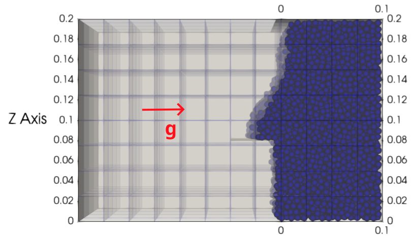
First, during the loading stage (\(0-6\) s), \(8849\) particles are inserted with a temperature of \(20°C\) in a rectangular box. In this part of the simulation, \(g = 9.81 \mathbf{e_x}\) because we insert the particles from the side of the box. When particles are sufficiently static, we use a solid surface to even out the particles on the side of the packed bed. Then, a second solid surface is placed on the side to close the box and keep the particles in place for the next stage of the simulation. Just before the end of this stage, at \(t = 5.95\) s, the kinetic energy of the packed bed is \(3\times10^{-10}\) J, which is lower than the \(1\times10^{-7}\) J criterion used by Beaulieu for a stable packed bed.

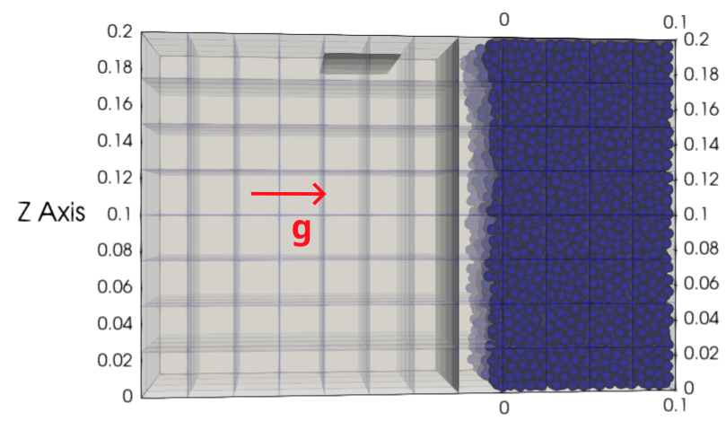
The second stage (\(6-7\) s) is where gravity is changed to \(g = -9.81 \mathbf{e_z}\) to be in the same direction as the experiment from Beaulieu [1]. We let the particle bed restructure for \(1\) s. At \(t = 6.95\) s, the kinetic energy of the packed bed is \(1\times10^{-9}\) J.

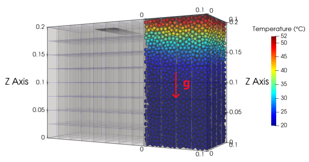
Finally, during the heating stage (\(7-4000\) s), the temperature of a solid surface placed on top on the packed bed is set to \(53°C\) and the particles are heated through this top wall. During this last part of the simulation, particle motion is disabled.

Parameter File

Mesh

The domain is a rectangular box with dimensions \(0.3\times0.1\times0.2\) meters and is made using the deal.ii grid generator.

subsection mesh
  set type               = dealii
  set grid type          = subdivided_hyper_rectangle
  set grid arguments     = 3,1,2 : -0.2 , 0.0 , 0.0 : 0.1 , 0.1 , 0.2 : false
  set initial refinement = 2
end

Insertion Info

In the loading stage, particles are inserted through the side of the box, with a temperature of \(20°C\). This initial temperature was chosen to match the experimental data.

subsection insertion info
  set insertion method                               = volume
  set inserted number of particles at each time step = 3400
  set insertion frequency                            = 10000
  set insertion box points coordinates               = -0.199, 0.001, 0.001 : -0.03, 0.099, 0.199
  set insertion distance threshold                   = 1.5
  set insertion maximum offset                       = 0.6
  set insertion prn seed                             = 17
  subsection initial temperature function
    set Function expression = 20
  end
end

Lagrangian Physical Properties

The \(8849\) particles are mono-dispersed, with a diameter of \(6.4\) mm.

The physical properties of the steel particles, the walls, and the interstitial gas were chosen to match those used by Beaulieu in her simulation. However, their Young’s moduli were set to be \(10\) times higher than those used by Beaulieu. This adjustment was made to ensure that our simulation reproduces the experimental porosity of \(42\%\) observed in the packed bed.

subsection lagrangian physical properties
  set g                        = 0.0, 0.0 , -9.81
  set number of particle types = 1
  subsection particle type 0
    set size distribution type            = uniform
    set diameter                          = 6.4e-3
    set number of particles               = 8849
    set density particles                 = 7747
    set young modulus particles           = 50e6
    set poisson ratio particles           = 0.29
    set restitution coefficient particles = 0.8
    set friction coefficient particles    = 0.7
    set rolling friction particles        = 0.02
    set real young modulus particles      = 200e9
    set thermal conductivity particles    = 42
    set specific heat particles           = 464
    set microhardness particles           = 3e9
    set surface slope particles           = 0.056
    set surface roughness particles       = 19.e-9
    set thermal accommodation particles   = 0.7
  end
  set young modulus wall           = 50e6
  set poisson ratio wall           = 0.33
  set restitution coefficient wall = 0.8
  set friction coefficient wall    = 0.7
  set rolling friction wall        = 0.02
  set real young modulus wall      = 100e9
  set thermal conductivity wall    = 250
  set microhardness wall           = 1.8e9
  set surface slope wall           = 0.056
  set surface roughness wall       = 0.1e-9
  set thermal accommodation wall   = 0.7
  set thermal conductivity gas     = 0.027
  set specific heat gas            = 1006
  set dynamic viscosity gas        = 1.85e-5
  set specific heats ratio gas     = 1
  set molecular mean free path gas = 68.e-9
end

Model Parameters

For the first two stages, the model parameters are defined as:

subsection model parameters
  subsection contact detection
    set contact detection method                = dynamic
    set dynamic contact search size coefficient = 0.9
    set neighborhood threshold                  = 1.3
  end
  subsection load balancing
    set load balance method = frequent
    set frequency           = 100000
  end
  set particle particle contact force method = hertz_mindlin_limit_overlap
  set rolling resistance torque method       = constant_resistance
  set particle wall contact force method     = nonlinear
  set integration method                     = velocity_verlet
  set solver type                            = dem_mp
end

For the heating of the particles, the parameter disable position integration is set to true to freeze the particles in place by disabling the time-integration of the particles’ velocity and position. This allows for the use of a larger time step for the evolution of the temperature, as collisions no longer need to be resolved. Since the particles remain stationary, load balancing is also no longer necessary.

subsection model parameters
  subsection contact detection
    set contact detection method                = dynamic
    set dynamic contact search size coefficient = 0.9
    set neighborhood threshold                  = 1.3
  end
  set particle particle contact force method = hertz_mindlin_limit_overlap
  set rolling resistance torque method       = constant_resistance
  set particle wall contact force method     = nonlinear
  set integration method                     = velocity_verlet
  set solver type                            = dem_mp
  set disable position integration           = true
end

Solid Objects

Three solid surfaces are used in this example. The first one is the one used to heat the packed bed from \(7\) s to \(4000\) s, with a temperature of \(53°C\). The second one is used to even the particles on the side of the packed bed. The last one closes the box to maintain the particles within it when the direction of the gravity is changed. The second and third walls are both set to adiabatic, meaning that they are insulated and do not provide any heat transfer.

subsection solid objects
  subsection solid surfaces
    set number of solids = 3
    subsection solid object 0
      subsection mesh
        set type               = gmsh
        set file name          = square-top.msh
        set simplex            = true
        set initial refinement = 0
      end
      subsection translational velocity
        set Function expression = 0 ; 0 ; 0
      end
      subsection angular velocity
        set Function expression = 0 ; 0 ; 0
      end
      set thermal boundary type = isothermal
      subsection temperature
        set Function expression = if(t>7,53,20)
      end
    end
    subsection solid object 1
      subsection mesh
        set type               = gmsh
        set file name          = square-rake.msh
        set simplex            = true
        set initial refinement = 0
      end
      subsection translational velocity
        set Function expression = if(z<0.19,0,if(t<3.6,-0.5,0)) ; 0 ; if(t>1.6 && z<0.19,0.1,0)
      end
      subsection angular velocity
        set Function expression = 0 ; 0 ; 0
      end
      set center of rotation    = 0 , 0 , 0
      set thermal boundary type = adiabatic
    end
    subsection solid object 2
      subsection mesh
        set type               = gmsh
        set file name          = square-side.msh
        set simplex            = true
        set initial refinement = 0
      end
      subsection translational velocity
        set Function expression = if(t>3.6 && x<-0.005,0.5,0) ; 0 ; 0
      end
      subsection angular velocity
        set Function expression = 0 ; 0 ; 0
      end
      set center of rotation    = -0.2 , 0 , 0
      set thermal boundary type = adiabatic
    end
  end
end

Note

The results are quite sensitive to the position of the side wall (square-side.msh), so it could probably be set more precisely for more accurate results.

Simulation Control

For the loading stage:

subsection simulation control
  set time step         = 2.5e-5
  set time end          = 6
  set log frequency     = 2000
  set output frequency  = 2000
  set output path       = ./output/
  set output boundaries = true
end

For the stage where gravity is changed:

subsection simulation control
  set time step         = 2.5e-5
  set time end          = 7
  set log frequency     = 2000
  set output frequency  = 2000
  set output path       = ./output/
  set output boundaries = true
end

For the heating stage:

subsection simulation control
  set time step         = 1
  set time end          = 4007
  set log frequency     = 10
  set output frequency  = 10
  set output path       = ./output/
  set output boundaries = true
end

Running the Simulation

This simulation is launched in three steps. First the particles are loaded with:

mpirun -np 4 lethe-particles load-packed-bed.prm

Then, the direction of gravity is changed with:

mpirun -np 4 lethe-particles flip-packed-bed.prm

Finally, we run the simulation to heat the particles:

mpirun -np 4 lethe-particles heat-packed-bed.prm

Note

In this example, the three stages require respectively around 16 minutes, 2 minutes and 2 minutes on 4 cores.

Post-processing

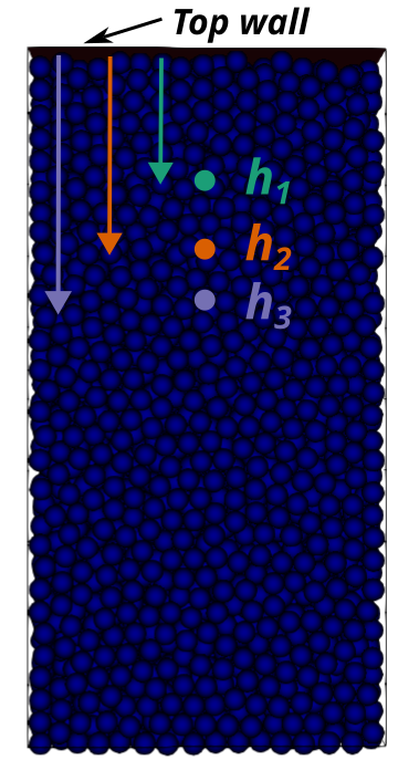
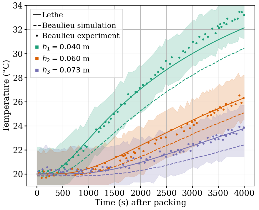
A Python post-processing code bed-postprocessing.py is provided with this example. It is used to compare the temperature of the packed-bed at three different heights \(h_1 = 4.0\) cm, \(h_2 = 6.0\) cm and \(h_3 = 7.3\) cm (\(h = 0.0\) cm corresponds to the top wall), with the results obtained experimentally and numerically by Beaulieu for stainless steel.

The post-processing code can be run with the following command. The argument is the folder which contains the .prm file.

  python3 bed-postprocessing.py  --folder ./

Important

You need to ensure that lethe_pyvista_tools is working on your machine. Click here for details.

Results

The following figure compares the temperature of the packed-bed at three different heights \(h_1 = 4.0\) cm, \(h_2 = 6.0\) cm and \(h_3 = 7.3\) cm, with the results obtained by Beaulieu for stainless steel.

The results show good agreement with the experimental and numerical results of Beaulieu but still undershoot a bit the temperature at \(h_1 = 4.0\) cm compared to the experimental data. Our temperature curves are slightly higher than the ones numerically obtained by Beaulieu due to the hertz contact radius used instead of the analytical one, as in Beaulieu’s work. The higher Young’s modulus employed also gives better results.

It has been noticed while experimenting with the model that the simulation results are highly sensitive to the loading method and to the wall friction coefficient. The following figure shows the results of the simulation with the friction coefficient wall set to \(1.0\) instead of \(0.7\).

This friction coefficient wall allows to fit the experimental data better but it is debatable whether a friction coefficient of \(1.0\) is realistic to model the Styrofoam walls used in the experiment. Also, other parameters like the rolling friction should have probably been adjusted as well to fit the experimental properties.

Note

Since the simulation results are highly sensitive to the loading, they may vary a bit from one computer to another.

Possibilities for Extension

• Reproduce the experimental and numerical results of Beaulieu for other particle types, such as glass beads and aluminum alloys beads.

Reference

[1] (1,2)

C. Beaulieu, “Impact de la ségrégation granulaire sur le transfert de chaleur dans un lit rotatif,” (Order No. 28990310), Ph.D. thesis, Polytechnique Montréal, 2020. Available: https://www.proquest.com/dissertations-thèses/impact-de-la-ségrégation-granulaire-sur-le/docview/2626891455/se-2.