Bubble detachment in shear flow

This example simulates the detachment of a growing bubble of air in a liquid shear flow.

Features

• Solver: lethe-fluid (Q1-Q1)

• Two phase flow handled by the Cahn-Hilliard-Navier-Stokes (CHNS) approach

• Modification of the unit of length of the problem using the dimensionality option

• Mobility coefficient setting for advective problems with CHNS solver

• Parametric sweep on the shear rate of the fluid

• Post-processing of the quantities of interest (detachment time and volume) and plots of the contour of the bubble at detachment

Files Used in This Example

All files mentioned below are located in the example’s folder (examples/multiphysics/bubble-detachment-shear-flow).

• Parameter file: bubble-detachment-shear-flow.prm

• Postprocessing Python script: multiple_folders_bubble_detachment_post_processing.py (using the functions of functions_bubble_detachment_post_processing.py)

• Parametric sweep generation files : generate_cases_locally.py, launch_lethe.sh and launch_lethe_cluster.py

Description of the Case

Bubble detachment in shear flow plays a key role in multiphase flows, where shear forces influence the separation of air bubbles from surfaces. This process is important in industries like petroleum engineering, where bubble behavior affects oil extraction, and chemical processing, where it impacts mixing and mass transfer. In this example, we simulate an air bubble in water under shear flow, highlighting how shear forces drive detachment from the interface.

The problem consists of a rectangular box of length \(L = 12 \ \text{mm}\), height \(H = 5 \ \text{mm}\) and thickness \(l = 5 \ \text{mm}\). The liquid phase flows from left to right following a Couette profile, that is determined with a given shear rate. At the bottom wall, there is a circular air inlet of radius \(R_0 = 0.5 \ \text{mm}\). Air is injected from this inlet following a Poiseuille profile. As the time passes, the bubble, which is initialized as a semi-sphere of radius \(R_0\), grows, until the shear force from the surrounding liquid and the buoyancy force detach it.

The computational domain with relevant boundary conditions is described in the following figure (not to scale):

2D slice of the domain of the bubble detachment in a shear flow

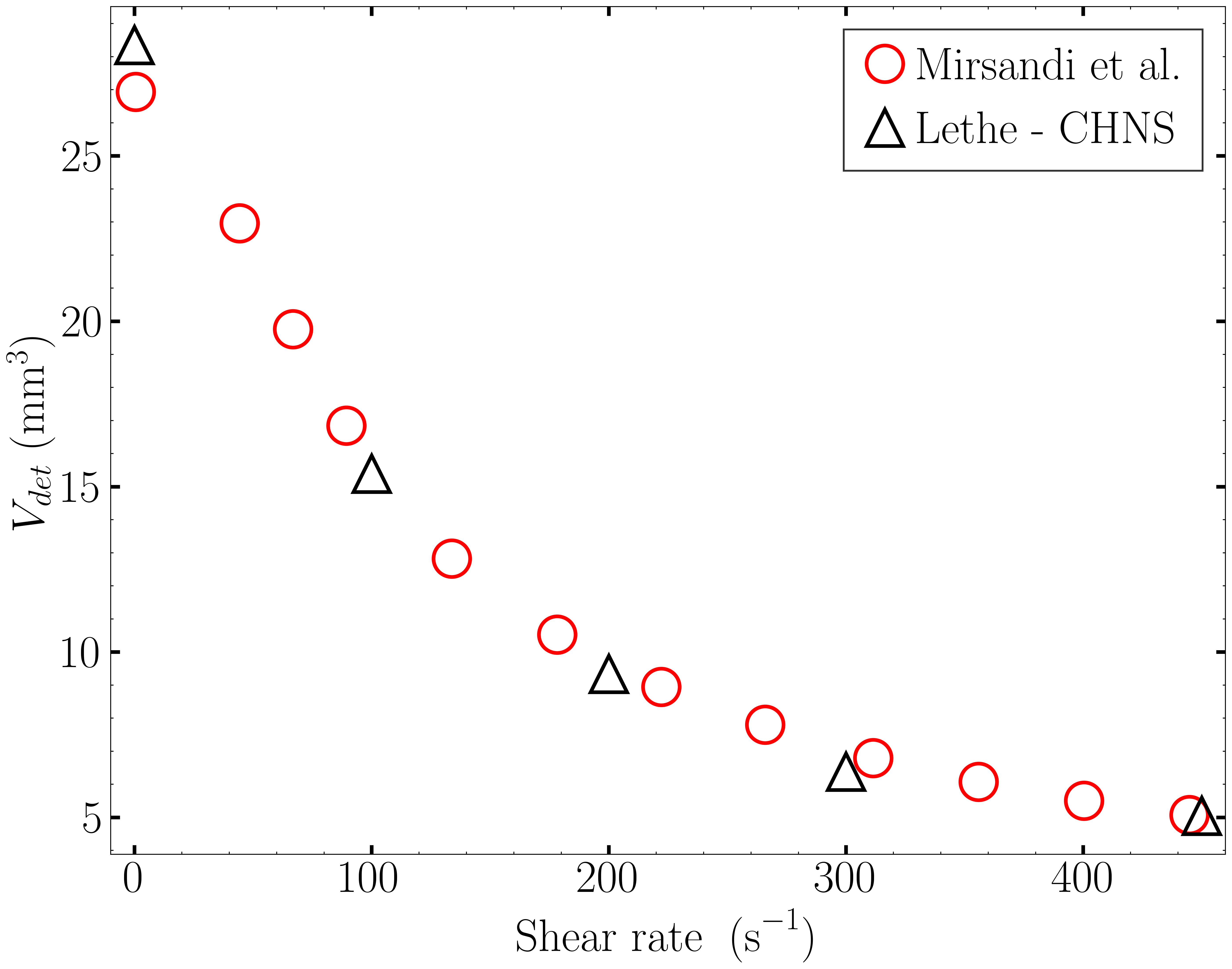
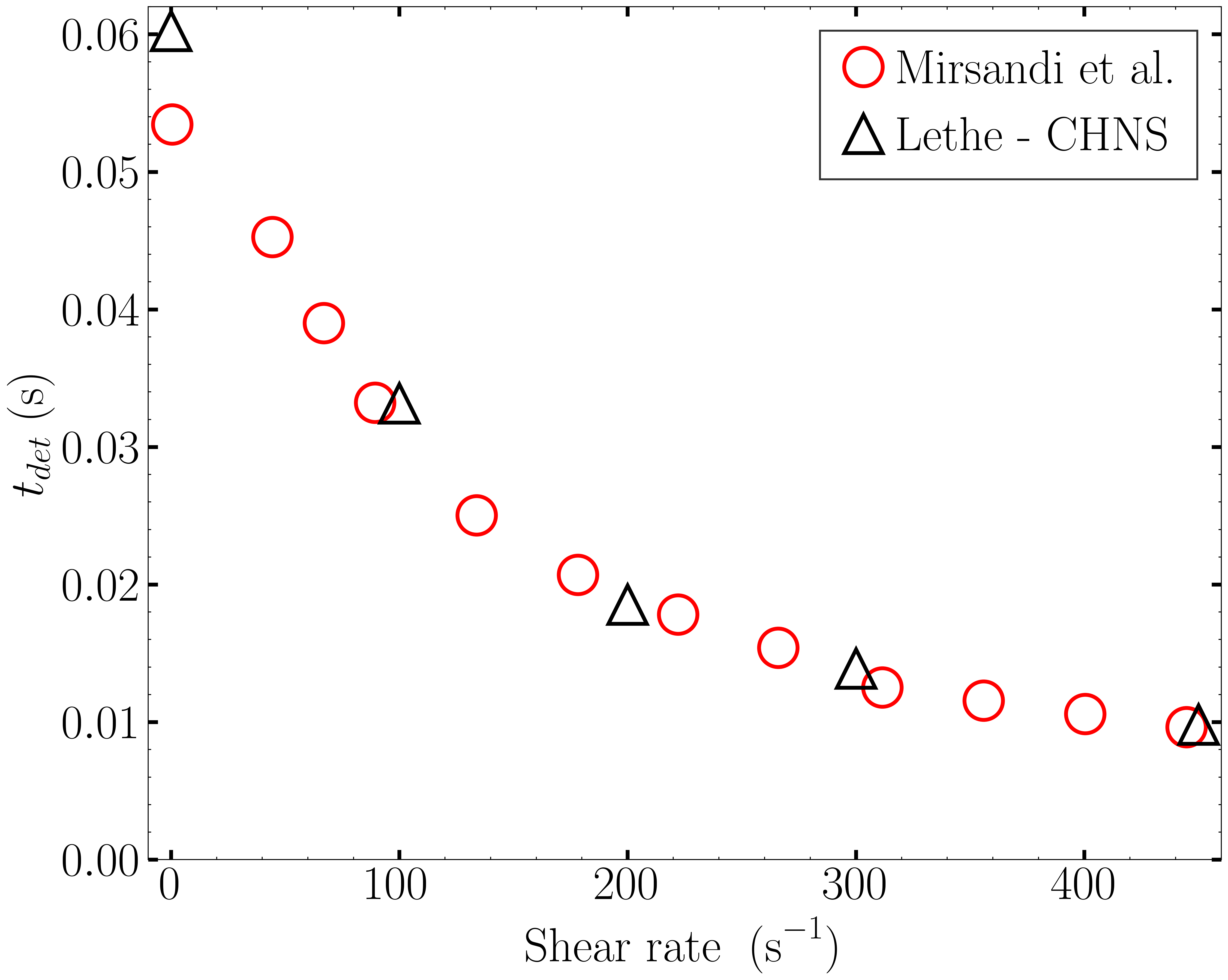
The quantity of interest of this problem is the detachment time \(t_\text{det}\). It is defined as the last time where the number of closed contour defined by a phase order field \(\phi=0\) (indicating a liquid-gas interface) is equal to 1. From this, we derive the detachment volume \(V_\text{det}\), which is the bubble volume at \(t_\text{det}\). We perform numerous simulations by changing the shear rate and compute the detachment times and volumes using the python scripts provided. Those results are then compared to the results from Mirsandi et al. [1] Below, all the parameters are set for a simulation whose shear rate is \(S = 450 \ \text{s}^{-1}\). Detailed instructions on how to generate the parameters files automatically for the parametric sweep are given in the Running the Simulation section of this example.

Parameter File

Simulation Control

Time integration is handled by a 2nd order backward differentiation scheme (bdf2), for a \(0.5 \ \text{s}\) simulation time with an initial time step of \(5 \times 10^{-7} \ \text{s}\). Time-step adaptation is enabled using adapt = true and the max cfl is \(0.9\). output boundaries is set to true to get a .vtu file containing the indices of the boundaries of the domain. The maximum time step is computed using the capillary time step condition given below:

\[\Delta t < \Delta t_\sigma = \sqrt{\frac{(\rho_a+\rho_l)\Delta x^3}{4\pi\sigma}}\]

where \(\rho_a\) and \(\rho_l\) are the densities of the gas and the liquid phases, respectively, \(\Delta x\) is the minimum cell size of the mesh and \(\sigma\) is the surface tension coefficient.

subsection simulation control
  set method            = bdf2
  set output name       = article-3d
  set output frequency  = 15
  set output path       = ./outputs/output/
  set time end          = 0.5
  set adapt             = true
  set max cfl           = 0.9
  set time step         = 5e-7
  set max time step     = 7.9784e-06 # Capillary timestep condition
  set output boundaries = true
end

Multiphysics

The multiphysics subsection is used to enable the cahn hilliard solver. Note that the fluid dynamics are solved by default.

subsection multiphysics
  set cahn hilliard = true
end

Dimensionality

The dimensionality subsection is used to define the length scale of the simulation as \(0.001 \ \text{m} = 1 \ \text{mm}\). This setting helps with the convergence of the solver.

Note

When using the dimensionality parameters, the problem and the physical properties are rescaled using the new units specified by the user. This means that physical properties need to be given in SI units and they will automatically be rescaled. The resulting fields (velocity and pressure for instance) will also be rescaled accordingly. The other subsections: source term, initial conditions and boundary conditions are not affected by the dimensionality parameters. Thus, any dimensioned parameter contained in these subsections need to be rescaled accordingly by the user.

subsection dimensionality
  set length = 0.001 # meter
end

Mesh

In the mesh subsection, we specify the mesh used in this example. The grid arguments are specified so the origin of the coordinate system is located at one sixth of \(L\), in the middle of the transversal direction and on the bottom wall. The subdivisions are such that the cells are close to a square shape.

subsection mesh
  set type               = dealii
  set grid type          = subdivided_hyper_rectangle
  set grid arguments     = 9,3,3 : -2,0,-2.5 : 10,5,2.5 : true
  set initial refinement = 3
end

Mesh Adaptation

The mesh adaptation section controls the dynamic mesh adaptation. Here, we choose phase_cahn_hilliard as the refinement variable. The maximum and minimum refinement levels are respectively set to \(6\) and \(3\) with the number of initial refinement steps set to \(4\) to adequately capture the interface at the beginning. This ensures the physics close to the interface to be well resolved, while keeping a coarse cell size far from the interface. The mesh refinement frequency is set to \(3\) because the refinement operation is expensive on 3D meshes. The fraction refinement and fraction coarsening are set to keep a high level of refinement close to the interface.

subsection mesh adaptation
  set type                     = kelly
  set variable                 = phase_cahn_hilliard
  set fraction type            = fraction
  set max refinement level     = 6
  set min refinement level     = 3
  set frequency                = 3
  set fraction refinement      = 0.995
  set fraction coarsening      = 0.005
  set initial refinement steps = 4
end

Cahn-Hilliard

In the cahn hilliard subsection, we set the potential smoothing coefficient (soon to be deprecated) to \(0\). The interface thickness is set to be determined automatically based on the mesh size in the epsilon subsection. We also output the interface thickness for each time-step by setting the verbosity to verbose to know its exact value for the initial conditions.

subsection cahn hilliard
  set potential smoothing coefficient = 0
  subsection epsilon
    set method    = automatic
    set verbosity = verbose
  end
end

Initial Conditions

In the initial conditions subsection, we initialize both the fluid velocity in the uvwp subsection and the phase field in the cahn hilliard subsection.

First the velocity over the domain is initialized to that of a Couette flow of a given shear rate. The velocity profile of a Couette flow and the associated shear rate \(S\) are related as:

\[\mathbf{u}_\text{in,l}(y) = S\cdot y\mathbf{e}_x\]

Here, the initial conditions are those corresponding to \(S = 450 \ \text{s}^{-1}\). We multiply by \(1000\) because the unit length is the millimeter.

The chemical potential field is set to \(0\) uniformly. The air bubble is initialized as a semi-sphere centered with the air inlet with a radius equal to \(R_0\). This corresponds to the following phase profile at \(t = 0\):

\[\phi(x,y,z) = -\text{tanh}\left(\frac{R_0 - \sqrt{x^2 + y^2 + z^2}}{\sqrt{2}\epsilon}\right)\]

subsection initial conditions
  subsection uvwp
    set Function expression = 1000*2.25*(y/5);0;0;0
  end

  subsection cahn hilliard
    set Function expression = -tanh((5e-1 - sqrt(y*y + x*x + z*z))/(1.41*0.0418546));0
  end
end

Boundary Conditions

We need to set boundary conditions both for the fluid dynamics solver and the Cahn-Hilliard solver. For the latter, we impose a dirichlet boundary condition on the phase field on the lower wall. This acts like a clamping condition for the bubble, so it can not be dragged on the lower surface. All the other boundary conditions are assumed to be noflux, both for the phase and the chemical potential.

subsection boundary conditions cahn hilliard
  set number = 6
  subsection bc 0 # lower-walls
    set id   = 2
    set type = dirichlet
    subsection phi
      set Function expression = -tanh((5e-1 - sqrt(x*x + z*z))/(1.41*0.0346))
    end
  end
  subsection bc 1
    set id   = 1
    set type = noflux
  end
  subsection bc 2
    set id   = 0
    set type = noflux
  end
  subsection bc 3
    set id   = 3
    set type = noflux
  end
  subsection bc 4
    set id   = 4
    set type = noflux
  end
  subsection bc 5
    set id   = 5
    set type = noflux
  end
end

For the Navier-Stokes equations, we constrain the velocity to correspond to that of a Couette flow at the inlet (subsection bc 0) and the upper wall (subsection bc 1). Then, the velocity profile on the bottom wall (subsection bc 2) needs to be \(0\) outside of the air inlet and must correspond to a Poiseuille profile in the air inlet. We remind the expression of the Poiseuille velocity profile below:

\[\mathbf{u}_{\text{in,a}} = u_\text{max,a}\left(1-\frac{x^2+z^2}{R_0^2}\right)\mathbf{e}_y\]

This profile corresponds to a volumetric air flux \(Q = 500 \ \text{mm}^3\text{s}^{-1}\) so that \(u_\text{max,a} = \frac{2Q}{\pi R_0^2} = 1.2732 \ \text{m} \text{s}^{-1}\). Once again, we multiply by \(1000\) because the length scale is \(1\) millimeter.

The lateral walls (subsection bc 4 and subsection bc 3) are endowed with slip boundary conditions and the last boundary (subsection bc 5) is defined as an outlet, with a penalization constant \(\beta = 100\).

subsection boundary conditions
  set number = 6
  subsection bc 0 # fluid-inlet
    set id   = 0
    set type = function
    subsection u
      set Function expression = 1000*2.25*(y/5)
    end
  end
  subsection bc 1 # upper-walls
    set id = 3
    set type = function
    subsection u
      set Function expression = 1000*2.25
    end
  end
  subsection bc 2 # lower-walls : gas-inlet + no-slip
    set id   = 2
    set type = function
    subsection v
      set Function expression = if(x*x + z*z < 5e-1*5e-1,1000*1.2732395447351625*(1-(x*x+z*z)/(0.5*0.5)),0)
    end
    subsection u
      set Function expression = 0
    end
    subsection w
      set Function expression = 0
    end
  end
  subsection bc 3 # side-walls
    set id   = 4
    set type = slip
  end
  subsection bc 4 # side-walls
    set id   = 5
    set type = slip
  end
  subsection bc 5 # fluid-outlet
    set id   = 1
    set type = outlet
    set beta = 100
  end
end

Physical Properties

The physical properties subsection defines the physical properties of the fluids. In this example, we need first to define the properties of the surrounding liquid as that of water, hence the choice of \(\rho_0 = 1000 \ \text{kg}\cdot\text{m}^{-3}\) and \(\nu_0 = 1.0016 \times 10^{-6} \ \text{m}^2\cdot\text{s}^{-1}\). The gas in the bubble is air, whose physical properties are \(\rho_1 = 1.23 \ \text{kg}\cdot\text{m}^{-3}\) and \(\nu_1 = 1.455\times 10^{-5} \ \text{m}^2\cdot\text{s}^{-1}\) . Since we have a water-air interface, the surface tension coefficient is: \(\sigma = 0.073 \ \text{N}\cdot\text{m}^{-1}\).

In this problem, the radius of the bubble is below the critical radius (see Yue et al. [2]), which means the air bubble will diffuse in the liquid phase over the timescale of the problem if the mobility coefficient is not set adequately. Yue et al. derive a criterion for setting the mobility coefficient \(D\) that depends on the parameters of the problem. It is given below:

\[D = \frac{(S + S_a)R_0\epsilon}{\sigma}\]

where \(S\) is the shear rate related to the liquid flow, \(S_a\) is the shear rate related to the air flow, \(\epsilon\) is the interface thickness and \(\sigma\) is the surface tension coefficient. \(S_a\) is the only unknown, it is estimated as follows:

\[S_a = \frac{u_\text{max,a}}{2R_0}\]

subsection physical properties
  set number of fluids = 2
  subsection fluid 0 # Water (phase = 1)
    set kinematic viscosity = 1.0016e-06
    set density             = 1000
  end
  subsection fluid 1 # Air (phase = -1)
    set kinematic viscosity = 14.55e-6
    set density             = 1.23
  end
  set number of material interactions = 1
  subsection material interaction 0
    subsection fluid-fluid interaction
      set surface tension coefficient     = 0.073
      set cahn hilliard mobility model    = constant
      set cahn hilliard mobility constant = 2.8177e-08 # No diffusion on problem time-scale condition
    end
  end
end

Source Term

In the source term subsection, we define the gravitational acceleration. Since the unit length is the millimeter, the usual value of \(g\) needs to be multiplied by \(1000\).

subsection source term
  subsection fluid dynamics
    set Function expression = 0; -9810; 0; 0
  end
end

Post-processing

In order to compute the quantities of interest of the problem, we enable Lethe to post-process the phase field at every iteration (set output frequency = 1). The phase statistics and the flow rates are necessary to compute derived quantities to analyze the problem more in-depth.

subsection post-processing
  set verbosity        = quiet
  set output frequency = 1

  set calculate barycenter       = true
  set calculate phase statistics = true

  set calculate flow rate = true
end

Running the Simulation

The simulation may be run locally by calling lethe-fluid by invoking:

 mpirun -np 10 lethe-fluid jurins-law-2d.prm

to run the simulation using ten CPU cores.

Though we highly advise you to run the simulation on a computationnal cluster (such as Narval, Béluga, etc.). To do so, a python script (generate_cases_locally.py) is included to generate automatically the cases with the correct parameters and physical properties locally. The script works with a .prm template (bubble-detachment-shear-flow.prm) and a .sh file (launch_lethe.sh) containing the information to launch the simulation on Narval. To use the python script, invoke:

 python3 generate_cases_locally.py

This will generate all the directories corresponding to the different shear rates cases. The directories’ names contain important information on the parameters of the simulation, hence the obscure naming. It will also generate summary_sweep.dat which sums up the parameters of the different cases in one file.

Once the directories are copied on Narval, launch the simulations with launch_lethe_cluster.py.

For more information, you may visit How to Automatically Create and Launch Lethe Simulations.

Then, to post-process the results, you may use the provided multiple_folders_bubble_detachment_post_processing.py python script. It contains all the instructions inside to run it.

Results

In order to analyze the influence of the surrounding liquid on the detachment of the bubble, we run the simulations for different values of the shear rate: \(S \in [100,200,300,450]\). The detachment time and volume are then computed and compared to the results of Mirsandi et al. [1] in the following figure, which shows an excellent agreement. The result of the no-shear simulation was added to the plot for completion.

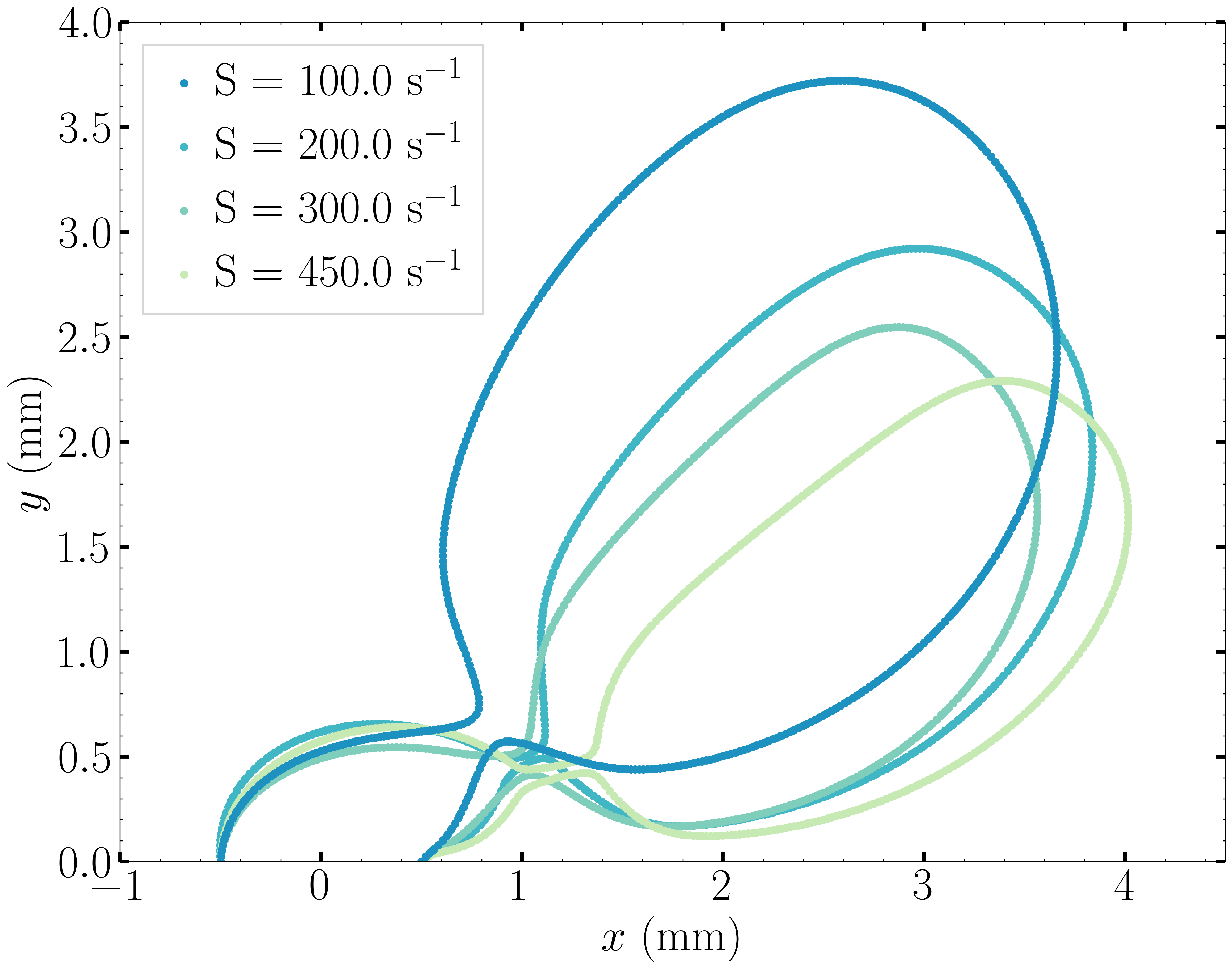
Below are the plots of the contour of the bubble in the plane \(z = 0\) when detachment occurs for different values of the shear rate.

The higher the shear rate, the more important the viscous drag as it can be observed above. The bubble is dragged in the direction of the movement of the fluid which flattens it, and brings it closer to the bottom wall. The volume enclosed by the contour is smaller, which is coherent with the values of detachment time and volumes computed before.

The video below displays the results for the case of \(S = 450 \ \text{s}^{-1}\)

Possibilities for Extension

• Non-newtonian case: extend the case to a non-newtonian liquid. This should yield fairly different results because of the high gradients of shear rate close to the bubble’s interface.

References

[1] (1,2)

H. Mirsandi, W. J. Smit, G. Kong, M. W. Baltussen, E. A. J. F. Peters, and J. A. M. Kuipers, ‘Bubble formation from an orifice in liquid cross-flow’, Chemical Engineering Journal, vol. 386, p. 120902, Apr. 2020, doi: 10.1016/j.cej.2019.01.181.

[2]

P. Yue, C. Zhou, and J. J. Feng, ‘Spontaneous shrinkage of drops and mass conservation in phase-field simulations’, Journal of Computational Physics, vol. 223, no. 1, pp. 1–9, Apr. 2007, doi: 10.1016/j.jcp.2006.11.020.