Rayleigh-Plateau Instability#
This example simulates the transition of a continuous jet to a droplet regime under the influence of a perturbation. The case simulated in this example corresponds to the case J1 in absence of gravity from the work of Denner et al. [1] with the Weber number \(\mathrm{We} = 50\) and the Ohnesorge number \(\mathrm{Oh} = 0.1\).
Features#
Solver:
lethe-fluidConservative Level-Set (CLS)
Unsteady problem handled by an adaptive BDF2 time-stepping scheme
Bash scripts to write, launch, and postprocess multiple cases
Python scripts for postprocessing data
Files Used in This Example#
All files mentioned below are located in the example’s folder (examples/multiphysics/rayleigh-plateau-instability).
Case generation and simulation launching Bash script:
rayleigh-plateau-launch.shParameter file for case generation:
rayleigh-plateau-J1-We050-Oh0_10.tplParameter file the for 2D case with an excitation amplitude (\(\delta_0\)) of \(0.2\):
rayleigh-plateau-J1-We050-Oh0_10_delta0_20/rayleigh-plateau-J1-We050-Oh0_10_delta0_20.prmParameter file for the 3D case with \(\delta_0 = 0.3\):
3D-delta0_30/rayleigh-plateau-J1-3D.prmPostprocessing Python script for breakup lengths extraction:
rayleigh-plateau-postprocess.pyPostprocessing Python script for code to code comparison:
rayleigh-plateau-compare.pyPostprocessing Bash script:
rayleigh-plateau-postprocess.shReference results from Denner et al. [1] for code-to-code verification (\(\mathrm{We}=50\) and \(\mathrm{Oh}=0.1\)):
denner-et-al-2022-We050.csv
Description of the Case#
Surface tension is renowned for its stabilizing effects, yet it also serves a disruptive role in various applications, such as inkjet printing. There, the surface tension plays a pivotal role in breaking up the continuous inkjet into droplets, governed by the destabilizing mechanism on the interface between the air and the ink known as the Rayleigh-Plateau instability.
In this example, the Rayleigh-Plateau instability is simulated through a continuous glycerol jet that undergoes a perturbation of different excitation amplitudes. The velocity imposed at the jet inlet takes the following form:
where \(U\) is the initial uniform velocity of the jet, \(\delta_0\) is the excitation amplitude, \(f = \frac{\kappa U}{2 \mathrm{\pi} R_\mathrm{inlet}}\) is the excitation frequency with \(\kappa = \frac{2 \mathrm{\pi} R_\mathrm{inlet}}{\lambda}\) the dimensionless wavenumber (\(\lambda\) is the wavelength) and \(R_\mathrm{inlet}=1.145 \times 10^{-3} \; \mathrm m\) the inlet radius. Lastly, \(t\) is the time.
Note
It is assumed that at the initial state the air is static \(\left(\mathbf{u}_\mathrm{air} = \mathbf{0} \; \mathrm{m\, s^{-1}}\right)\).
The following figure displays the initial state:

|
Note
In this example, the gravity contribution is not considered \(\left(Fr = \frac{u}{\sqrt{g R_\mathrm{inlet}}} \rightarrow \infty \right)\).
Parameter File#
The parameter file for the case of \(\delta_0 = 0.20\) is shown below.
Simulation Control#
The time integration is handled by a 2nd-order backward differentiation scheme (bdf2) with a maximum time step of \(\Delta t = 4.4 \times 10^{-5} \; \text{s} \approx \Delta t_\sigma\) which corresponds to the capillary time-step constraint (see capillary wave example).
subsection simulation control
  set method                         = bdf2
  set time end                       = 0.08
  set time step                      = 4.4e-5
  set adapt time step to respect CFL = true
  set max cfl                        = 0.75
  set max time step                  = 4.4e-5
  set output name                    = rayleigh-plateau
  set output frequency               = 5
  set output path                    = ./output_delta0_20/
end
Multiphysics#
The multiphysics subsection is used to enable the CLS solver.
subsection multiphysics
  set cls  = true
end
Physical Properties#
In the physical properties subsection, we define the jet fluid (fluid 1) as presented for case J1 in Denner et al. [1] The viscosity is deduced from the imposed Ohnesorge number \(\left(\mathrm{Oh}=\frac{\mu_1}{\sqrt{\sigma\rho_1 R_\mathrm{inlet}}} \right)\) value of \(0.1\). The ambient fluid (fluid 0) is defined such that the density \(\left(\frac{\rho_1}{\rho_0} = 10^3 \right)\) and dynamic viscosity \(\left(\frac{\mu_1}{\mu_0} = 10^2\right)\) ratios are respected. A fluid-fluid type of material interaction is also defined to specify the surface tension model. In this case, it is set to constant (default value) with the surface tension coefficient (\(\sigma\)) set to \(0.0674 \; \mathrm{N \, m^{-1}}\).
subsection physical properties
  set number of fluids = 2
  subsection fluid 0
    set density             = 1.196
    set kinematic viscosity = 2.54e-4
  end
  subsection fluid 1
    set density             = 1196
    set kinematic viscosity = 2.54e-5
  end
  set number of material interactions = 1
  subsection material interaction 0
    set type = fluid-fluid
    subsection fluid-fluid interaction
      set surface tension coefficient = 0.0674
    end
  end
end
Mesh#
In the mesh subsection, we define a subdivided hyper rectangle with appropriate dimensions. The mesh is initially refined \(7\) times to ensure adequate definition of the interface.
subsection mesh
  set type               = dealii
  set grid type          = subdivided_hyper_rectangle
  set grid arguments     = 4 , 1 : 0, -0.01145 : 0.0916, 0.01145 : true
  set initial refinement = 7
end
Mesh Adaptation#
In the mesh adaptation subsection, we dynamically adapt the mesh using the phase as refinement variable. We choose \(5\) as the min refinement level and \(8\) as the max refinement level. We set initial refinement steps = 4 to adapt the mesh to the initial value of the CLS field.
subsection mesh adaptation
  set type                     = adaptive
  set error estimator          = kelly
  set variable                 = phase
  set fraction type            = fraction
  set max refinement level     = 8
  set min refinement level     = 5
  set fraction refinement      = 0.99
  set fraction coarsening      = 0.001
  set initial refinement steps = 4
end
Initial Conditions#
In the initial conditions, we define the initial condition as presented in the figure above.
The uniform jet velocity \((U = 1.569 \; \mathrm{m \, s^{-1}})\) corresponds to \(\mathrm{We}=\frac{\rho_1 R_\mathrm{inlet} U^2}{\sigma}=50\).
subsection initial conditions
  set type = nodal
  subsection uvwp
    set Function constants  = U=1.569
    set Function expression = if(y^2 <= 1.3110e-6, U, 0); 0; 0
  end
  subsection CLS
    set Function expression = if(y^2 <= 1.3110e-6, 1, 0)
    subsection projection step
      set enable = true
    end
  end
end
Boundary Conditions#
In the boundary conditions subsection, the inlet velocity perturbation is specified as described in the description of the case with \(\kappa = 0.7\). Note that we set beta = 0 for the outlet boundary condition to allow for fluid reentry. Otherwise, the default behavior of the outlet boundary condition will be to penalize fluid reentry which will affect the flow.
subsection boundary conditions
  set number = 3
  subsection bc 0
    set id   = 0
    set type = function
    subsection u
      set Function constants  = U=1.569, delta=0.2, kappa=0.7, r=1.145e-3
      set Function expression = if (y^2 <= 1.3110e-6, U*(1 + delta*sin(kappa*U*t/r)), 0)
    end
  end
  subsection bc 1
    set id                 = 2
    set type               = periodic
    set periodic id        = 3
    set periodic direction = 1
  end
  subsection bc 2
    set id                 = 1
    set type               = outlet
    set beta               = 0
  end
end
Boundary Conditions CLS#
Lasty, in the boundary conditions CLS subsection we ensure that fluid 1 is at the inlet. The other boundary conditions are default outlets.
subsection boundary conditions CLS
  set number = 3
  subsection bc 0
    set id   = 0
    set type = dirichlet
    subsection dirichlet
      set Function expression = if(y^2 <= 1.3110e-6, 1, 0)
    end
  end
  subsection bc 1
    set id                 = 2
    set type               = periodic
    set periodic id        = 3
    set periodic direction = 1
  end
  subsection bc 2
    set id   = 1
    set type = none
  end
end
Running the Simulation#
We can call lethe-fluid for each \(\delta_0\) value. For \(\delta_0 = 0.20\), this can be done by invoking the following command:
to run the simulation using fourteen CPU cores. Feel free to use more CPU cores.
Warning
Make sure to compile Lethe in Release mode and run in parallel using mpirun. This simulation takes \(\sim \, 20\) minutes on \(14\) processes.
Tip
If you want to generate and launch multiple cases consecutively, a Bash script (rayleigh-plateau-launch.sh) is provided. Make sure that the file has executable permissions before calling it with:
where "{0.05 0.1 0.15 0.2 0.25 0.3 0.35 0.4 0.5 0.6}" is the sequence of \(\delta_0\) values of the different cases.
Note
An additional -ne argument can be added at the end before running the script if you do not wish to extract all breakup lengths but only generate the comparison figure.
Results#
Simulation Results#
The video below displays the results for the case of \(\delta_0 = 0.2\).
Satellite Droplets#
The video below displays the apparition of satellite droplets (secondary droplets) at at higher excitation amplitudes. Here, \(\delta_0 = 0.3\).
This 3D simulation was simulated using the 3D-delta0_30/rayleigh-plateau-J1-3D.prm parameter file.
Note
Note that in these simulations, the mass is not perfectly conserved. It can be observed that the satellite droplets are fading away. This will be worked on in future updates.
Code to Code Comparison#
We compare the dimensionless breakup length \(\left(\frac{L_\mathrm{b}}{R_\mathrm{jet}}\right)\) with the simulation results from Denner et al. [1] \(L_\mathrm{b}\) is the breakup length defined as the shortest distance from the nozzle (inlet) to the tip of the continuous jet.
The results can be postprocessed using the provided Bash script (rayleigh-plateau-postprocess.sh). Make sure that the file has executable permissions before calling it with:
with denner-et-al-2022-We050.csv being the path to the reference data csv file.
Important
You need to ensure that the lethe_pyvista_tools is working on your machine. Click here for details.
This script extracts breakup lengths of the cases while excluding the satellite droplets. The script then calculates an average \(L_\mathrm{b}\) which is used to evaluate the dimensionless breakup length of the jet.
Note
The script ignores the first 2 breakups of the jet as they as considered not part of the periodical behavior.
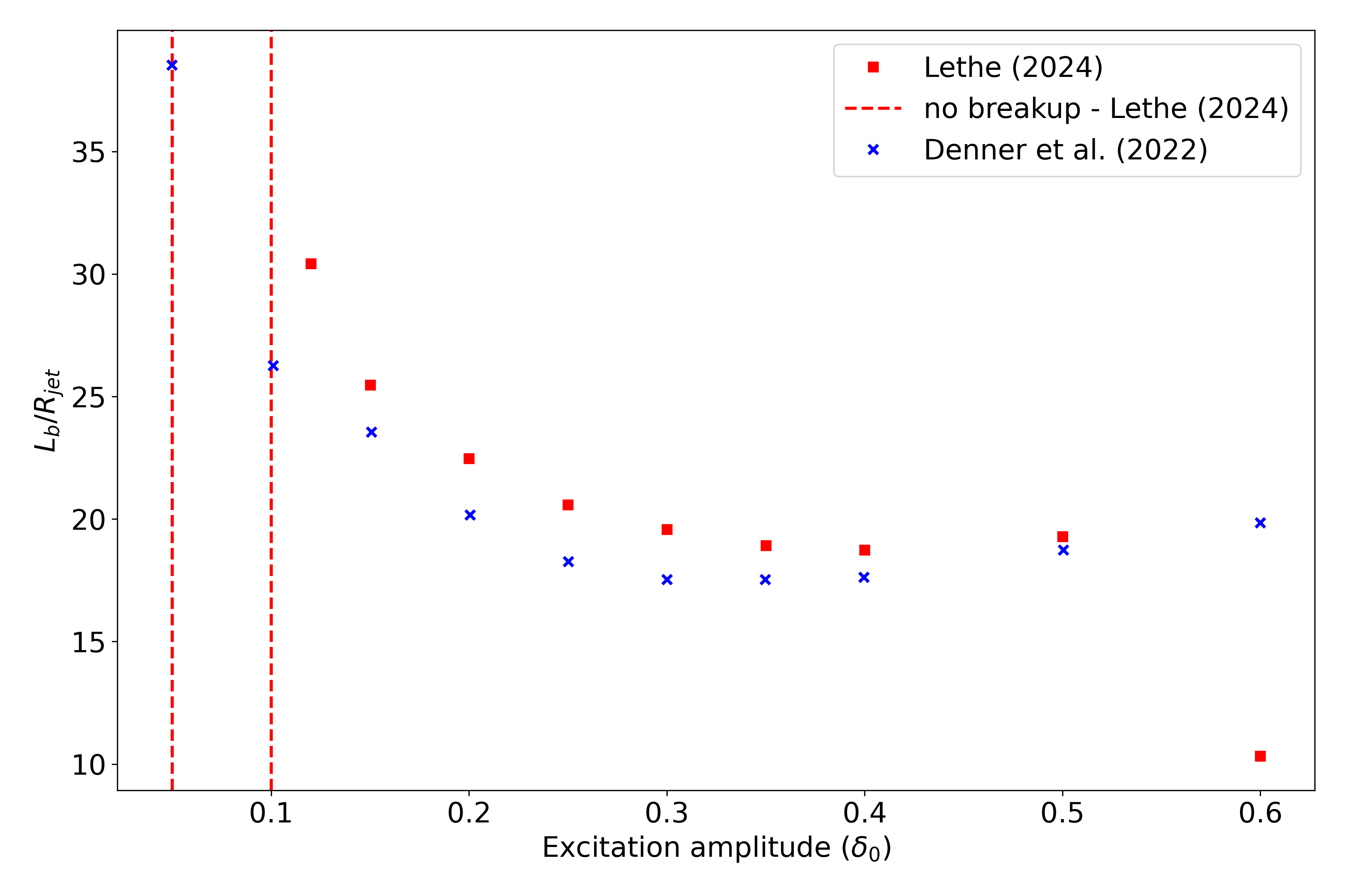
|
As it can be seen above, for \(\delta_0 \leq 0.1\), we observe no breakup. The jet stabilizes despite the perturbation. An additional case was studied at \(\delta_0 = 0.12\) to check the increasing stabilizing tendency of the jet for lower excitation amplitude values. We also observe that none of the other evaluation points match with the work of Denner et al. [1] These differences can be due to the 2D simulation setup used to generate the results of Lethe, while the ones of Denner et al. are obtained from a 3D setup. At \(\delta_0 = 0.6\), a huge difference is observed. This is due to the way the satellite droplets are formed. As opposed to previous simulations, the satellite droplets are formed from the broken-off part of the jet, decreasing significantly \(L_\mathrm{b}\) as displayed in the video below. This might have not been the case in the work of Denner et al. [1]