3D Dam-Break with an Obstacle

This example simulates a dam-break experiment from the Maritime Research Institute Netherlands (MARIN) [1].

Warning

This example displays the need for improvement of low-viscosity fluid flow simulation of the current numeric model. Further work will be done to improve this aspect of the model.

Features

• Solver: lethe-fluid (Q1-Q1)

• Two phase flow handled by the Volume-of-Fluids (VOF) approach with phase fraction filtration

• Mesh adaptation using phase fraction

• Unsteady problem handled by an adaptive BDF1 time-stepping scheme

• The use of a python script for post-processing data

Files Used in This Example

All files mentioned below are located in the example’s folder (examples/multiphysics/3d-dam-break).

• Experimental data file: experimental_data.txt

• Geometry file: tank_with_obstacle.geo

• Mesh file: tank_with_obstacle.msh

• Parameter file: 3d-dam-break.prm

• Postprocessing Python script: 3d-dam-break_postprocess.py

Description of the Case

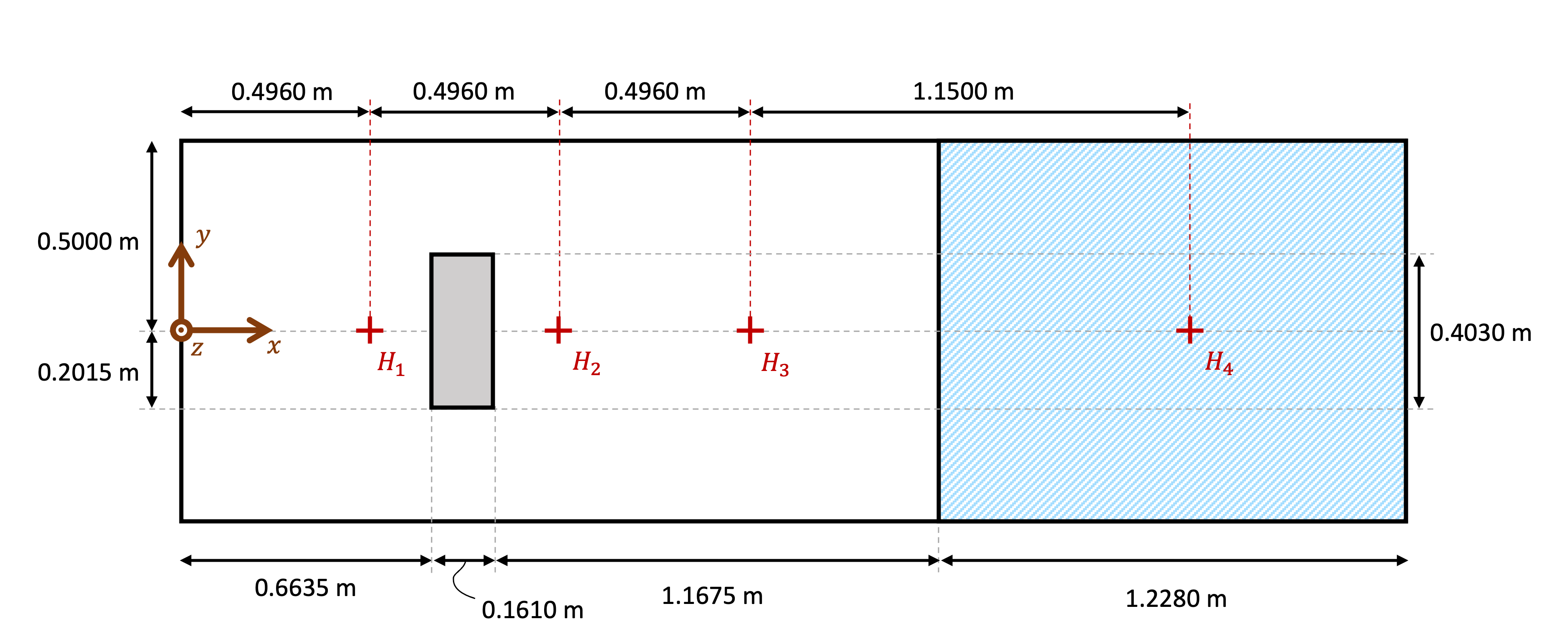
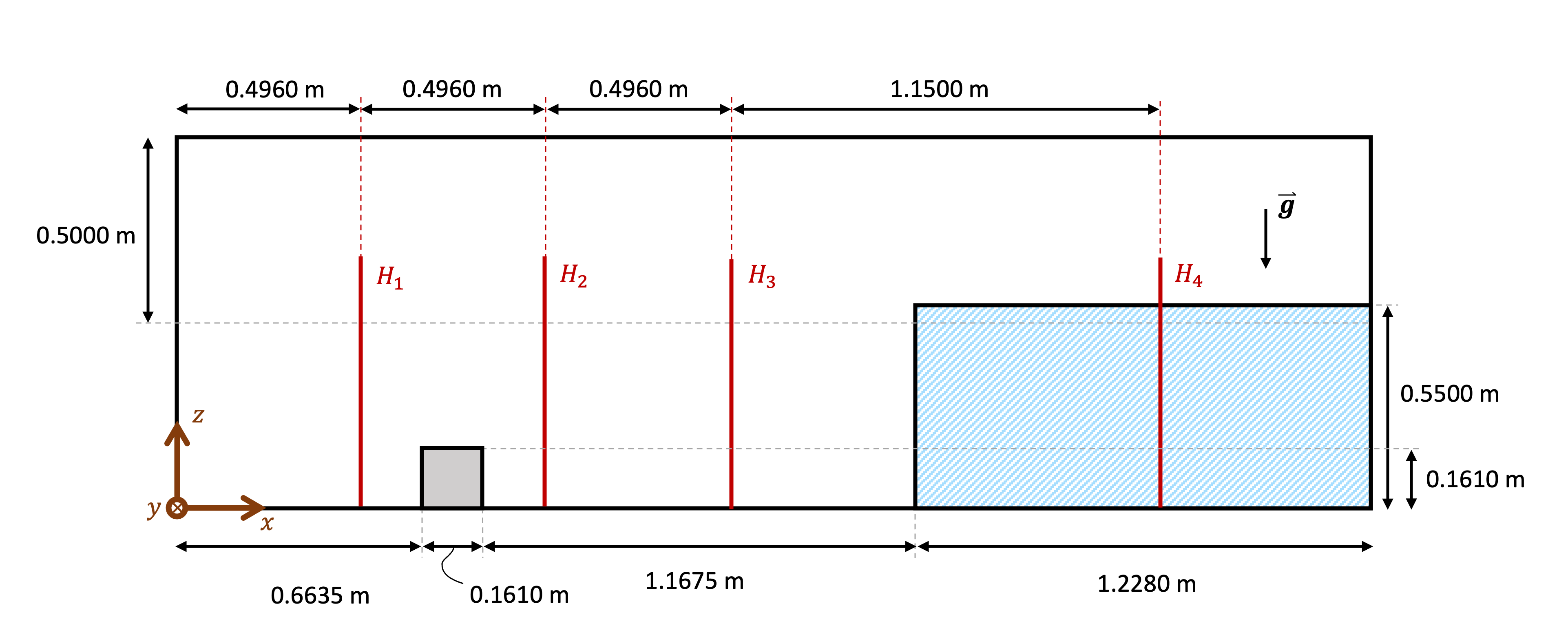
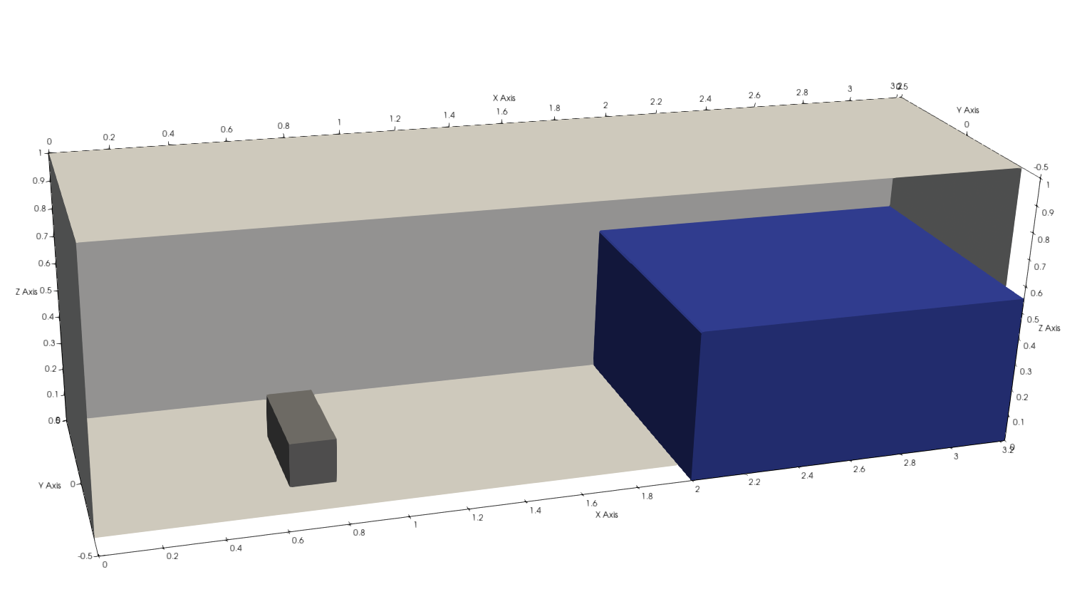
For this example, the simulated fluids are water and air. Initially, the water is at rest on the right side of the tank (represented in dashed blue lines in the figures below). At \(t = 0 \ \text{s}\), the gate opens instantaneously and the water starts flowing under the action of gravity, \(\mathbf{g} = (-9.81 \ \mathbf{j}) \frac{\text{m}}{\text{s}^2}\). The tank in which this experiment happens has the following dimensions: \(3.22 \times 1.00 \times 1.00 \ \text{m}\). On all boundaries, slip conditions were applied. On the left side of the tank, a rectangular box-shaped obstacle is presented (colored in grey in the figures).

Along the x-axis, the water height is measured at 4 different positions. These positions are represented by red crosses in the figure below.

Initial state top view

Initial state side view

Initial state in 3D

Parameter File

Simulation Control

Time integration is handled by a 1st order backward differentiation scheme (bdf1), for a \(6 \ \text{s}\) simulation time with an initial time step of \(0.001 \ \text{s}\). Time-step adaptation is enabled using adapt=true and the max CFL is \(0.8\).

Note

This example uses an adaptive time-stepping method, where the time-steps are modified during the simulation to keep the maximum value of the CFL condition below the given threshold (0.5).

subsection simulation control
  set method                       = bdf1
  set time end                     = 6
  set time step                    = 0.001
  set adapt                        = true
  set max cfl                      = 0.8
  set output name                  = 3d-dam-break
  set output frequency             = 5
  set output path                  = ./output/
  set adaptative time step scaling = 1.05
  set output boundaries            = true
end

Multiphysics

The multiphysics subsection enables to turn on (true) and off (false) the physics of interest. Here VOF is chosen. Note that the fluid dynamics are solved by default.

subsection multiphysics
  set VOF = true
end

Physical Properties

The physical properties subsection defines the physical properties of the fluids. In this example, we need two fluids with densities of \(1.204 \ \frac{\text{kg}}{\text{m}^3}\) (air) and \(1000 \ \frac{\text{kg}}{\text{m}^3}\) (water). However, the current numerical model was not able to solve with the real dynamic viscosities of the fluids. Therefore, they were altered in order to run the simulation.

Warning

Altering the dynamic viscosities of the fluids will surely have an impact on the results. We will show this impact in the results section.

subsection physical properties
  set number of fluids = 2
  subsection fluid 0
    set density             = 1.204
    set kinematic viscosity = 0.01516
  end
  subsection fluid 1
    set density             = 1000
    set kinematic viscosity = 0.001
  end
end

Initial Conditions

In the initial conditions subsection, we need to define the interface between the two fluids. We define this interface by using a function expression in the VOF subsection of initial conditions. A projection step is applied to ensure a smooth definition of the initial condition.

subsection initial conditions
  set type = nodal
  subsection uvwp
    set Function expression = 0; 0; 0; 0
  end

  subsection VOF
    set Function expression = if (x>1.992 & z<0.55 & y>=-0.5, 1, 0)
    subsection projection step
      set enable           = true
      set diffusion factor = 1
    end
  end
end

Source Term

In the source term subsection, we define the gravitational acceleration.

subsection source term
  subsection fluid dynamics
    set Function expression = 0;0;-9.81;0
  end
end

VOF

In the VOF subsection, we select the tanh filter to filter the phase fraction and get a more defined interface. We set the value of beta to 10.

subsection VOF
  subsection phase filtration
    set type   = tanh
    set beta   = 10
  end
end

Mesh

In the mesh subsection, we specify the mesh used in this example. The structured mesh used in this example can be generated from the tank.geo file using Gmsh. The initial refinement is set to \(3\).

subsection mesh
    set type                 = gmsh
    set file name            = tank.msh
    set initial refinement   = 3
end

Mesh Adaptation

The mesh adaptation section controls the dynamic mesh adaptation. Here, we choose phase and pressure as the refinement variables. The maximum and minimum refinement levels are respectively set to \(4\) and \(2\).

subsection mesh adaptation
  set type                     = kelly
  set variable                 = phase, pressure
  set fraction type            = fraction
  set max refinement level     = 4
  set min refinement level     = 2
  set frequency                = 2
  set fraction refinement      = 0.999, 0.4
  set fraction coarsening      = 0.001, 0.05
  set initial refinement steps = 5
end

Running the Simulation

We call the lethe-fluid by invoking:

mpirun -np $number_of_CPU_cores lethe-fluid 3d-dam-break.prm

Warning

Make sure to compile Lethe in Release mode and run in parallel using mpirun. This simulation took \(\approx\) 17 hours on 64 processes (runned on the Narval cluster).

Results

The following video shows the results of the simulation:

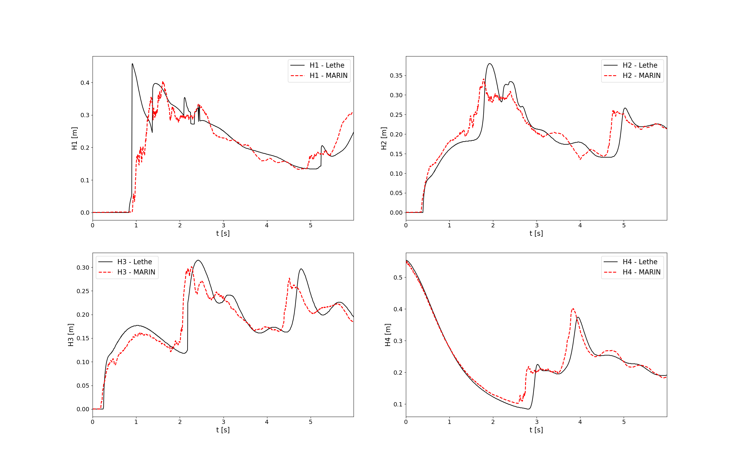
In the following figure, we compare the water height evolution at the 4 positions mentioned in the description of the case section with the experimental results obtained from MARIN (available here):

Comparison of the water height evolution

As we can see, the simulated general evolution of the height seems to follow the experimentation results. However, on all 4 subplots, we notice that the height is overestimated. We also notice a slight shift to the right for \(H2\), \(H3\), and \(H4\) evolutions. These observations may be explained by the “highly viscous air” (fluid 0) that acts as an obstacle to the free flow of the water. Additionally, fluid 1 representing the water is 1000 times more viscous than regular water. With these results, we can see that the model needs to be improved to be able to accurately simulate low-viscosity fluids such as air. Furthermore, we observe that the wave formed at the impact with the obstacle doesn’t collapse the right way due to the lack of compressibility of the air being simulated.

References

[1]

R. Issa and D. Violeau, “Test-case 2, 3D dambreaking, Release 1.1,” ERCOFTAC SPH Eur. Res. Interest Community SIG Électricité Fr. Lab. Natl. Hydraul. Environ., 2006, Accessed: Dec. 07, 2022. [Online]. Available: https://www.spheric-sph.org/tests/test-02.