Granuheap

This example simulates the flow of a cohesive granular material inside a Granuheap instrument using the discrete element method (DEM). For more detailed information on the concepts and physical meaning of the parameters in Lethe, we strongly recommend visiting DEM parameters.

Features

• Solvers: lethe-particles

• Three-dimensional problem

• Moving solid surface

• GMSH grids

• Multi-case simulations

Files Used in This Example

All files mentioned below are located in the example’s folder (examples/dem/3d-granuheap).

• Mesh file: cylinder.msh and support.msh

• Python file to generate mesh files: generate_meshes.py

• Parameters files for the problem: granuheap.prm and granuheap_multicase.prm

• Post-processing python files: post_processing.py, post_processing_multicase.prm and post_processing_functions.py.

Description of the Case

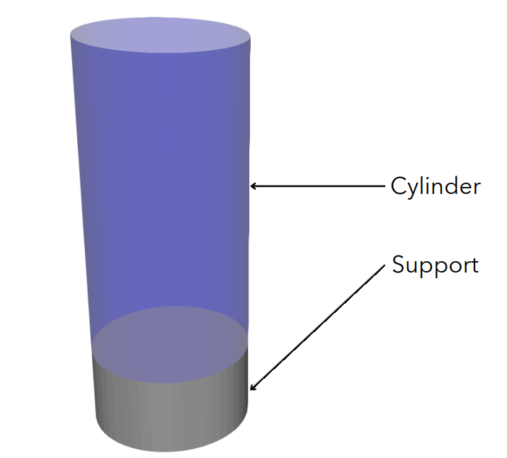
This example simulates the flow of wet sand during a Granuheap experiment. First, the packing of particles is generated by inserting particles inside a cylinder. After 1.6s, the cylinder rises, and the particles can flow freely, producing a heap. We compare the numerical results with our experimental results. To remain consistent with the Granuheap experiment, we use the same geometry in our simulations: a cylinder of 0.01m in diameter. For more information aboutt the Granuheap procedures, visit the Granuheap web page. To match our experimental results, we test multiple combinations of parameters in our simulations. We use the work of Hu et al. [1] as a basis to choose which contact properties will create those combinations.

Generate Mesh Files

To generate the cylinder.msh and support.msh files, we used the generate_meshes.py file. The two functions take as input the bottom’s position (x0), the radius, the number of points in the circumference, and the height.

cylinder(x0, radius, n_points, height)
support(x0, radius, n_points, height)

In this case, the cylinder has a height of 0.02m and a radius of 0.005m. The support has a height of 0.005m and has the same diameter as the cylinder. We fix the number of points in the circumference at 50 for both the cylinder and the support.

cylinder(-0.005, 0.005, 50, 0.02)
support(-0.01 ,0.005 ,50, 0.005)

Mesh files can be generated using the following command.

python3 generate_meshes.py

Note

GMSH is needed to generate mesh files. See GMSH website for installation and Introduction on How to Use GMSH for more information.

Parameter File

Mesh

The domain we simulate is a rectangular box measuring \(0.045\times0.02\times0.02\) meters, made using the deal.ii grid generator. The grid is refined 6 times using the set initial refinement parameter so that the cell size is approximately 1.5 times the largest particle diameter value.

subsection mesh
set type               = dealii
set grid type          = subdivided_hyper_rectangle
set grid arguments     = 3,1,1 : -0.010,-0.01,-0.01 : 0.035, 0.01,0.01 : true
set initial refinement = 6
end

Boundaries Conditions

The bottom of the domain is set as an outlet to allow the particles to leave the domain, thus reducing the computational time of the simulation.

subsection DEM boundary conditions
set number of boundary conditions = 1

subsection boundary condition 0
set boundary id         = 0
set type                = outlet
end
end

Lagrangian Physical Properties

The particles have a polydisperse size distribution with a density of 1922 \(kg/m^3\). 400 000 particles would be needed to approximately match the 2 g of sand used in the experiment. However, to reduce the simulation’s duration of this example, we insert only 200 000 particles.

According to Hu et al. [1] the rolling friction and the surface energy parameters impact the final simulated angle of repose (AOR) the most. Thus, we simulate twelve combinations of those parameters. The rolling friction is between 0.3 and 0.7, and the surface energy is between 0.0010 and 0.0100. The granuheap.prm file of this example is specifically for a rolling friction of 0.5 and a surface energy of 0.0100.

The water volume fraction of the wet sand used in the experiment is 0.325 %. According to the work of Liefferink et al. [2], this water volume fraction matches an friction coefficient of 0.5. We use this value as a rough estimate of the friction coefficient for this example.

subsection lagrangian physical properties
set g                        = -9.81, 0, 0
set number of particle types = 1
subsection particle type 0
set size distribution type            = custom
set custom diameters                  = 1.02e-4 , 1.16e-4 , 1.33e-4 , 1.52e-4 , 1.75e-4 , 2.00e-4 , 2.29e-4 , 2.62e-4 , 3.01e-4 , 3.44e-4
set custom volume fractions           = 0.04 , 0.06 , 0.07 , 0.10 , 0.13 , 0.15 , 0.16 , 0.14 , 0.10 , 0.05
set number of particles               = 200000
set density particles                 = 1922
set young modulus particles           = 5.94e4
set poisson ratio particles           = 0.4
set restitution coefficient particles = 0.9
set friction coefficient particles    = 0.5
set rolling friction particles        = 0.5
set surface energy particles          = 0.01
end
set young modulus wall           = 1e7
set poisson ratio wall           = 0.33
set restitution coefficient wall = 0.9
set friction coefficient wall    = 0.5
set rolling friction wall        = 0.5
set surface energy wall          = 1e-4
end

Model Parameters

The JKR contact model is used in this case because it has be shown to correctly model particle agglomeration for wet sand [1] .

subsection model parameters
subsection contact detection
set contact detection method                = dynamic
set dynamic contact search size coefficient = 0.9
set neighborhood threshold                  = 1.3
end
subsection load balancing
set load balance method = frequent
set frequency           = 100000
end
set particle particle contact force method = hertz_JKR
set rolling resistance torque method       = constant_resistance
set particle wall contact force method     = JKR
set integration method                     = velocity_verlet
end

subsection restart
set checkpoint = true
set frequency  = 10000
set restart    = false
set filename   = dem
end

Particle Insertion

An insertion box is defined inside the cylinder. 10 000 particles are inserted every 9000 iterations. The size of the insertion box is chosen to ensure it is completely inside our cylinder which is smaller than our domain. Otherwise, particles will be lost during the insertion stage.

subsection insertion info
set insertion method                               = volume
set inserted number of particles at each time step = 10000
set insertion frequency                            = 9000
set insertion box points coordinates               = 0.015, -0.00325, -0.00325: 0.035, 0.00325, 0.00325
set insertion distance threshold                   = 1.2
set insertion maximum offset                       = 0.05
set insertion prn seed                             = 19
set insertion direction sequence                   =  1, 2, 0
end

Solid Object

We set the cylinder’s translational velocity to \(0.05 m/s\) after the particles were loaded, thus when the simulation time is larger than 1.6s.

subsection solid objects
subsection solid surfaces
set number of solids = 2
subsection solid object 0
subsection mesh
set type                   = gmsh
set file name              = cylinder.msh
set simplex                = true
end
subsection translational velocity
set Function expression = if (t>1.6, 0.05, 0) ; 0 ; 0
end
end
subsection solid object 1
subsection mesh
set type                   = gmsh
set file name              = support.msh
set simplex                = true
end
end
end
end

Simulation Control

The process duration lasts for 2.2 seconds. We output the simulation results in every 1000 iterations.

subsection simulation control
set time step         = 7.54e-6
set time end          = 2.2
set log frequency     = 1000
set output frequency  = 1000
set output path       = ./output/
set output name       = granuheap
set output boundaries = true
end

Running the Simulation

Running one case

A simulation with one set of values for the rolling friction and the surface energy can be launched using the following command:

mpirun -np 8 lethe-particles granuheap.prm

Note

This example needs a simulation time of approximately 5 hours on 12 processors using an AMD Ryzen 9 5900x 12-core processor.

Running multiple cases

Three files are needed to create and launch multiple simulations; generate_cases_locally.py, granuheap_multicase.prm and launch_lethe_locally.py. For more information, visit How to Automatically Create and Launch Lethe Simulations

In this case, we run 3 different values of rolling friction and 4 different values of surface energy, for a total of 12 simulations.

number_of_cases = 4

# Generation of data points
energy_first = 0.0010
energy_last = 0.0100
energy = np.linspace(energy_first, energy_last, number_of_cases)

rolling_friction_first = 0.3
rolling_friction_last = 0.7
rolling_friction = np.linspace(rolling_friction_first, rolling_friction_last, number_of_cases-1)

Simulations can be launched using the following commands:

python3 generate_cases_locally.py
python3 launch_lethe_locally.py

Post-processing

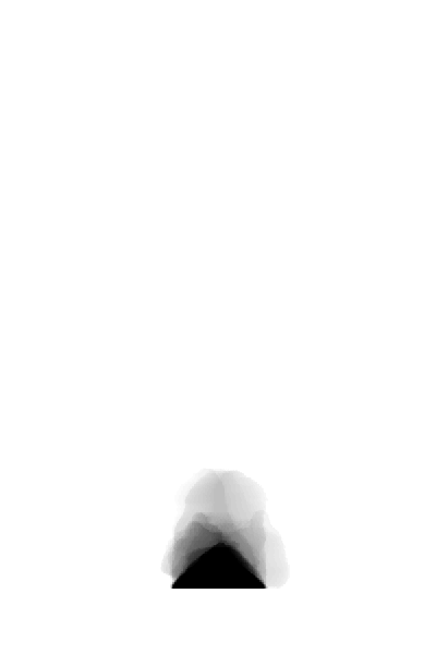
The Granuheap machine captures 16 pictures around the heap in a 180-degree arc. The images generate a map that distinguishes areas with constant particle presence (black), no particle presence (white), and varying particle presence (expressed through different shades of gray). The image below shows the map of the wet sand experiment and is provided as experimental_result.png

Running one case

To compare only one simulation with the experimental results, the post_processing.py file can be launched using the following command.

pvpython post_processing.py

The post-processing feature is launched using PvPython, the Python interface to the Paraview Software. It allows users to control ParaView with Python, thus without opening the user interface. PvPython can also run python scripts.

If the experimental file is not the one provided in this example, the exp_path, height_exp, and width_exp will need to be updated in the post_processing.py file.

# Path to the granuheap experimental result
exp_path = 'experimental_result.png'
# Name of simulation output (see OUTPUT NAME set in the simulation subsection of the parameter file)
num_output = 'granuheap'
# Output path (see OUTPUT PATH set in the simulation subsection of the parameter file)
out_path = 'output'
# Number of pixels in height and width of your experimental support (to adjust if you change experimental result)
height_exp = 60
width_exp = 85

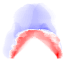
This file will generate a map of the simulation and subtract it from the experimental map to obtain the profile shape error. This error will be presented in a new image saved as image_difference.png. The picture below presents the profile shape error for a rolling friction of 0.5 and a surface energy of 0.0100.

This post_processing file will also output the Root Mean Square Error (RMSE) in the terminal.

Running multiple cases

For multiple cases, the post_processing_multicase.py file should be used using the following command.

pvpython post_processing_multicase.py

If the experimental file is not the one provided in this example, the exp_path, height_exp and width_exp will need to be updated in the post_processing_multicase.py file. The parameters’ names and values for each case can also be modified in the python file.

# Path of the granuheap experimental result
exp_path = 'experimental_result.png'
# Name of directory for each simulation (see CASE_PREFIX from the launch_lethe_locally.py file used)
num_name = 'wetsand'
# Name of simulation output (see OUTPUT NAME set in the simulation subsection of the parameter file)
num_output = 'granuheap'
# Output path (see OUTPUT PATH set in the simulation subsection of the parameter file)
out_path = 'output'
# Definition of variable parameters
parameter1_name = 'Surface Energy'
parameter1 = [0.0010, 0.0040, 0.0070, 0.0100]
parameter2_name = 'Rolling Friction'
parameter2 = [0.70, 0.50, 0.30]
# Number of pixels in height and width of your experimental support (to adjust if you change experimental result)
height_exp = 60
width_exp = 85

The code will generate a map for each simulation and then subtract them from the experimental map. Those errors will be presented in a new image saved as profile_shape_error.png.

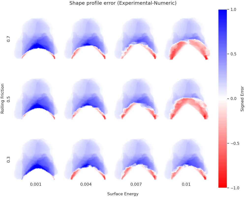
To confirm which simulation has the lowest error, an image saved as error_values_heatmap.png will present a heatmap of each simulation RMSE.

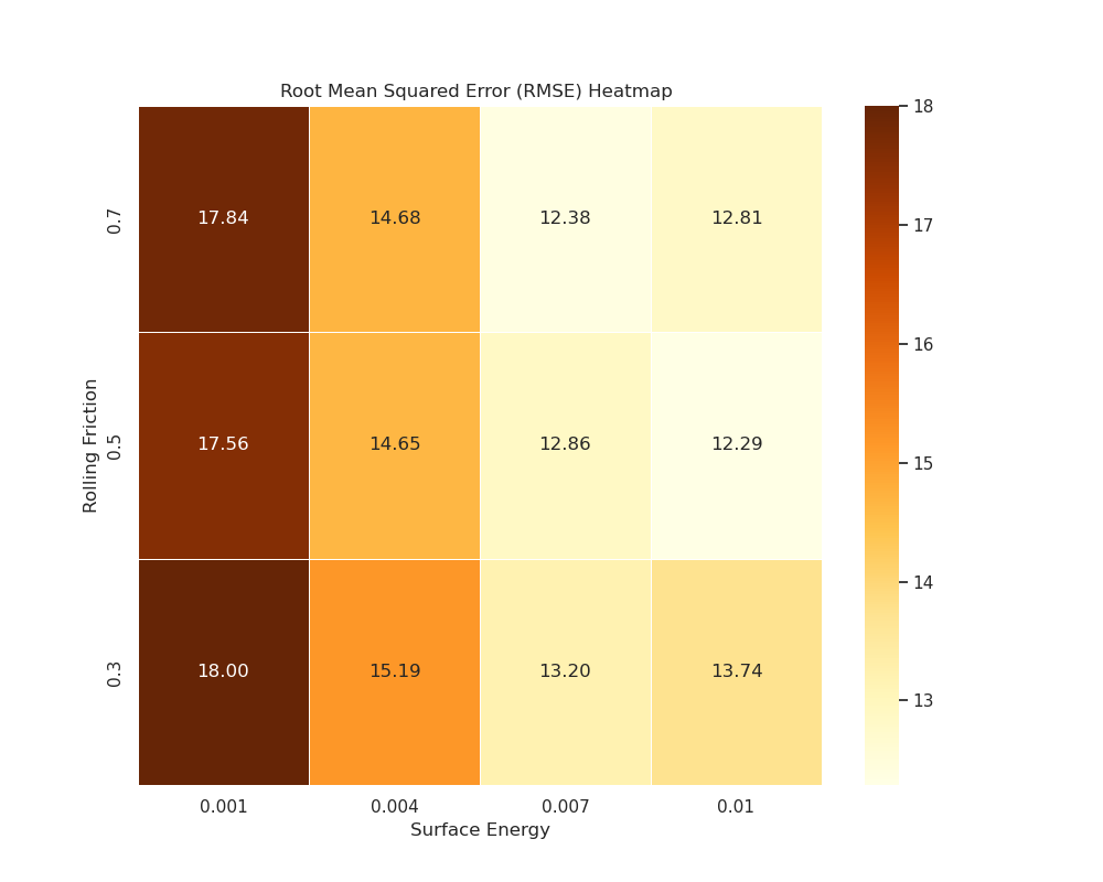
The lowest error is obtained when the rolling friction is 0.5 and the surface energy is 0.0100.

Note

The following libraries will be necessary to run post-processing files; PIL, numpy, matplotlib.pyplot, os, glob, scipy.interpolate and UnivariateSpline. The Paraview software is also needed.

Results

The video below presents the Granuheap simulation for a rolling friction of 0.5 and a surface energy of 0.0100.

Reference

[1] (1,2,3)

A. C. Hu, Z. Li, K. Mao, J. Tang, X. Wang, L. Zhang and J. Zhou, “Calibration of wet sand and gravel particles based on JKR contact model,” Powder Technology, vol. 397, Jan. 2022. doi: 10.1016/j.powtec.2021.11.049.

[2]

A. R.W. Liefferink, B. Weber and D. Bonn, “Ploughing friction on wet and dry sand,“ Physical Review E, vol. 98, Nov. 2018. doi: 10.1103/PhysRevE.98.052903.