Rayleigh-Taylor Instability

This example simulates the dynamic evolution of the single-mode Rayleigh-Taylor instability [1] by density contrast.

Features

• Solver: lethe-fluid

• Mesh adaptation using phase fraction

• Periodic boundary condition

• Unsteady problem handled by an adaptive BDF2 time-stepping scheme

• Monitoring mass conservation

• Interface sharpening

Files Used in This Example

All files mentioned below are located in the example’s folder (examples/multiphysics/rayleigh-taylor-instability).

• Parameter file for adaptive sharpening: rayleigh-taylor-instability-adaptive-sharpening.prm

• Parameter file for constant sharpening: rayleigh-taylor-instability-constant-sharpening.prm

• Postprocessing Python script: rayleigh-taylor_postprocess.py

Description of the Case

In this example, we simulate the Rayleigh-Taylor instability benchmark. In this benchmark, a dense fluid, as shown in the following figure, is located on top of a fluid with a smaller density.

The density ratio and viscosity ratio of the heavy (fluid 1) and light (fluid 0) fluids are

\[\rho_r = \frac{\rho_h}{\rho_l} = 3\]

\[\mu_r = \frac{\mu_h}{\mu_l} = 3\]

which result in Reynolds and Atwood numbers equal to

\[Re = \frac{\rho_h H \sqrt{H \bf{g} }}{\mu_h} = 256\]

\[At = \frac{\rho_r - 1}{\rho_r + 1} = 0.5\]

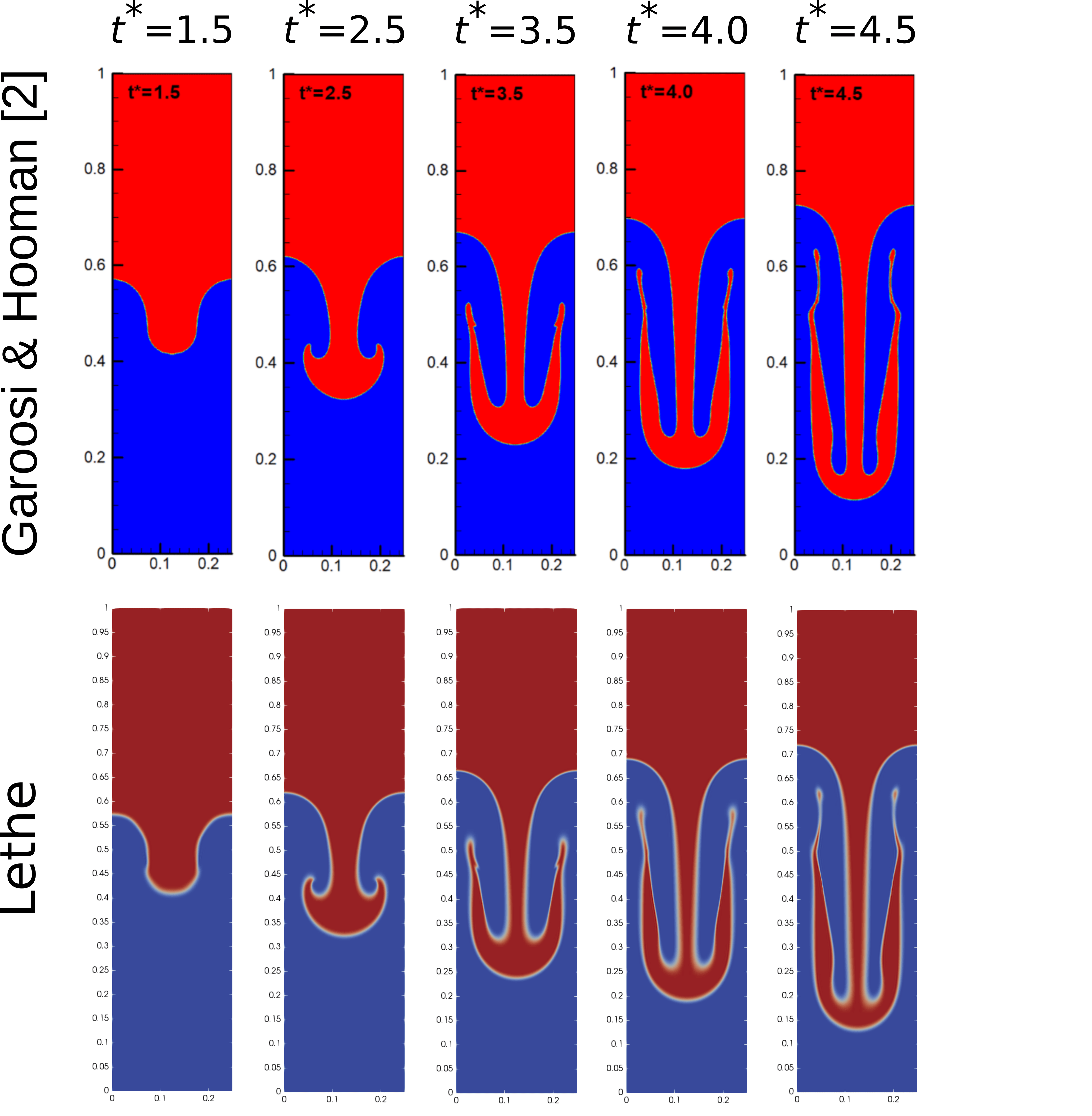
A perturbed interface defined as \(y = 2H + 0.1 H \cos{(2 \pi x / H)}\) separates the fluids. At the top and bottom boundaries, a no-slip boundary condition is applied, while on the left and right walls, a periodic boundary condition is used. The temporal evolution of the interface is visually compared with the simulations of Garoosi and Hooman [2] at dimensionless times (\(t^* = t \sqrt{\mathbf{g} / H}\)) of \(1.5\), \(2.5\), \(3.5\), \(4.0\) and \(4.5\). The temporal evolution of the spike and the bubble positions are then compared to the results of He et al. [1] The term “spike” refers to the lowest point of fluid 1 and the term “bubble” refers to the highest point of fluid 0.

Parameter File

Simulation Control

Time integration is handled by a 2nd order backward differentiation scheme (bdf2), for a \(0.75\, \text{s}\) simulation time with an initial time step of \(0.0002\) seconds. Time-step adaptation is enabled using adapt = true and the max CFL is \(0.8\).

Note

This example uses an adaptive time-stepping method, where the time-step is modified during the simulation to keep the maximum value of the CFL condition below a given threshold (\(0.9\) here). Using output control = time, and output time = 0.005 the simulation results are written every \(0.005\, \text{s}\).

subsection simulation control
  set method           = bdf2
  set time end         = 0.75
  set time step        = 0.001
  set adapt            = true
  set max cfl          = 0.8
  set output control   = iteration
  set output frequency = 10
  set output name      = rayleigh-taylor
  set output path      = ./output/
end

Multiphysics

The multiphysics subsection enables to turn on (true) and off (false) the physics of interest. Here VOF and fluid dynamics are chosen (fluid dynamics is true by default).

subsection multiphysics
  set VOF = true
end

Source Term

The source term subsection defines gravitational acceleration.

subsection source term
  subsection fluid dynamics
    set Function expression = 0 ; -9.81 ; 0
  end
end

Physical Properties

The physical properties subsection defines the physical properties of the fluid. In this example, we need two fluids with densities of \(100\) and \(300\) and with an equal kinematic viscosity (\(0.00153\)).

subsection physical properties
  set number of fluids = 2
  subsection fluid 0
    set density             = 100
    set kinematic viscosity = 0.00153
  end
  subsection fluid 1
    set density             = 300
    set kinematic viscosity = 0.00153
  end
end

Initial Conditions

In the initial conditions subsection, we need to define the interface between the heavy and light fluids. We define this interface by using a Function expression in the VOF subsection of the initial conditions. The interface between the two fluids is made smoother with the projection step parameter.

subsection initial conditions
  set type = nodal
  subsection uvwp
    set Function expression = 0; 0; 0
  end
  subsection VOF
    set Function expression = if (y>(0.5 + 0.1 * 0.25 * cos(2 *3.1415 * x / 0.25)) , 1, 0)
    subsection projection step
      set enable           = true
      set diffusion factor = 1
    end

  end
end

Mesh

In the mesh subsection we configure the simulation domain. The initial refinement of the mesh is equal to \(5\), but we use mesh adaptation to coarsen the mesh in cells far from the interface to improve the computation performance.

subsection mesh
  set type               = dealii
  set grid type          = subdivided_hyper_rectangle
  set grid arguments     = 1, 4 : 0.25, 1 : 0 , 0 : true
  set initial refinement = 5
end

Mesh Adaptation

The mesh adaptation section controls the dynamic mesh adaptation. Here, we choose phase as the refinement variable and \(5\) as the min refinement level. We set initial refinement steps = 4 to adapt the mesh to the initial value of the VOF field.

subsection mesh adaptation
  set type                     = kelly
  set variable                 = phase
  set fraction type            = fraction
  set max refinement level     = 7
  set min refinement level     = 5
  set frequency                = 1
  set fraction refinement      = 0.99
  set fraction coarsening      = 0.01
  set initial refinement steps = 4
end

Boundary Conditions

The boundary conditions applied on the left and right boundaries are periodic, while a noslip boundary condition is used for the top and bottom walls. In the definition of a periodic boundary, we need to specify the periodic_id and the periodic_direction (in this example, \(0\) which indicates the \(x\) direction).

subsection boundary conditions
  set number = 3
  subsection bc 0
    set id                 = 0
    set type               = periodic
    set periodic_id        = 1
    set periodic_direction = 0
  end
  subsection bc 1
    set id   = 2
    set type = noslip
  end
  subsection bc 2
    set id   = 3
    set type = noslip
  end
end

VOF

In the VOF subsection, we enable interface sharpening to reconstruct the interface and keep it sharp during the simulation. Note that here, we use the constant and adaptive methods for interface sharpening. Mass conservation results show that choosing a constant method does not affect the mass conservation significantly. Hence, the results of both methods are almost identical. For the constant sharpening we use:

subsection VOF
  subsection interface sharpening
    set enable              = true
    set threshold           = 0.5
    set interface sharpness = 1.5
    set frequency           = 25
    set type                = constant
  end
  subsection phase filtration
    set type      = tanh
    set verbosity = quiet
    set beta      = 10
  end
end

and for the adaptive sharpening:

subsection VOF
  subsection interface sharpening
    set enable                  = true
    set threshold               = 0.5
    set interface sharpness     = 1.5
    set frequency               = 25
    set type                    = adaptive
    set threshold max deviation = 0.2
    set max iterations          = 50
    set monitored fluid         = fluid 1
    set tolerance               = 1e-2
  end
  subsection phase filtration
    set type  = tanh
    set verbosity = verbose
    set beta = 10
  end
end

The phase filtration is enabled in this example. We refer the reader to the Volume of Fluid (Multiphase Flow) documentation for more explanation on the phase filtration.

Post-processing

In the post-processing subsection, the output of the mass of each fluid is enabled and allows to track to mass conservation throughout the simulation.

subsection post-processing
  set verbosity                   = verbose
  set calculate mass conservation = true
end

Running the Simulation

Call lethe-fluid by invoking:

mpirun -np 8 lethe-fluid rayleigh-taylor-instability-adaptive-sharpening.prm

to run the simulations using eight CPU cores. Feel free to use more.

Warning

Make sure to compile lethe in Release mode and run in parallel using mpirun. On \(8\) processes, this simulation takes \(\sim\) \(2\) minutes for the adaptive sharpening and \(\sim\) \(4\) minutes for constant sharpening.

Results and Discussion

In the following picture, the boundary between the two fluids is compared with (right) and without (left) projection step:

The following animation shows the results of this simulation:

In the following figure, we compare the simulation results with that of Garoosi and Hooman (2022) [2].

By invoking the rayleigh-taylor_postprocess.py postprocessing script found within the example folder with

python3 rayleigh-taylor_postprocess.py ./output/adaptive/

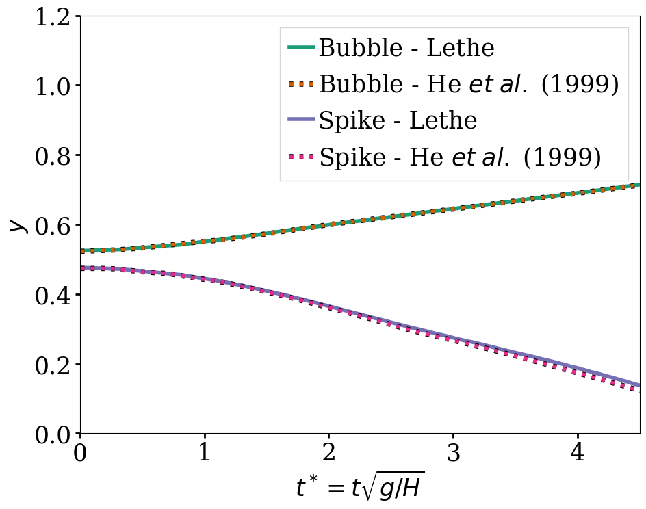
we compare the position of the spike and the bubble with the results of He et al. [1]

In the figure below, it can be seen that as \(t^*\) increases, there is a growing difference between the spike position of the current simulation and that of He et al. [1] Nevertheless, the bubble position follows the same evolution as the reference.

With higher levels of refinement, we can see better correspondence between the values. However, there is still a gap between the spike positions for larger values of \(t^*\).

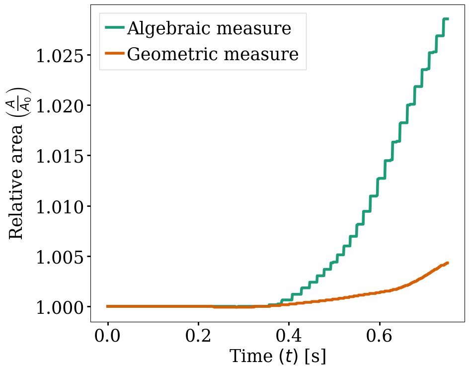
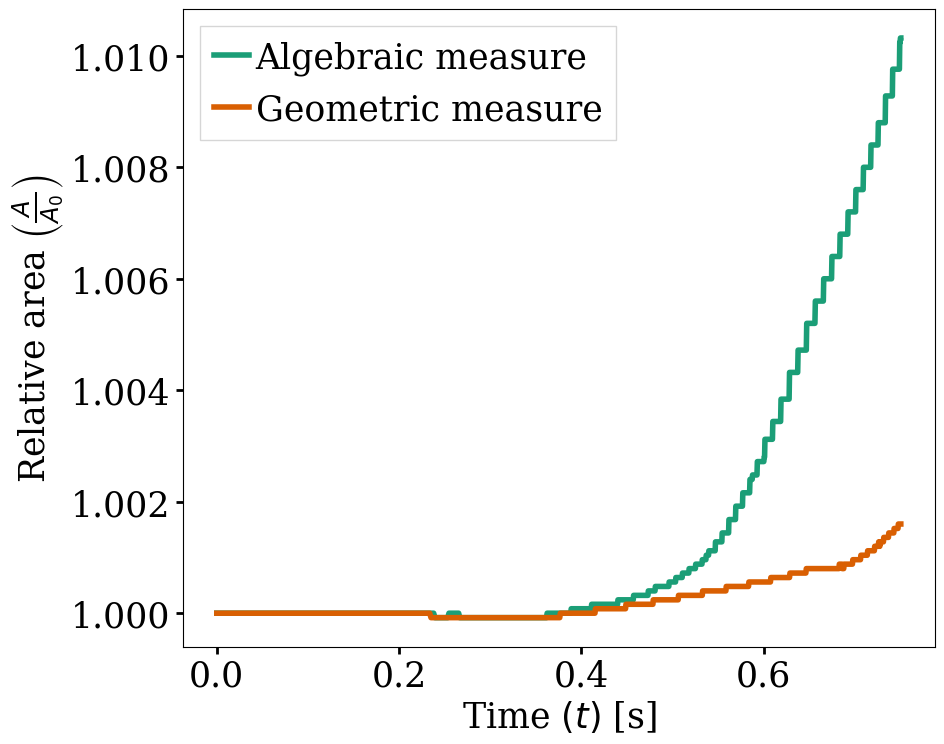
The following figures show the mass of fluid 1 throughout the simulation with a constant (left) and adaptive (right) interface sharpening.

References

[1] (1,2,3,4)

X. He, S. Chen, and R. Zhang, “A Lattice Boltzmann Scheme for Incompressible Multiphase Flow and Its Application in Simulation of Rayleigh–Taylor Instability,” J. Comput. Phys., vol. 152, no. 2, pp. 642–663, Jul. 1999, doi: 10.1006/jcph.1999.6257.

[2] (1,2)

F. Garoosi and K. Hooman, “Numerical simulation of multiphase flows using an enhanced Volume-of-Fluid (VOF) method,” Int. J. Mech. Sci., vol. 215, p. 106956, Feb. 2022, doi: 10.1016/j.ijmecsci.2021.106956.