Dense Pneumatic Conveying

This example simulates the dense pneumatic conveying of particles in a horizontal periodic pipe.

Features

• Solvers: lethe-particles and lethe-fluid-particles

• Three-dimensional problem

• Particle insertion according to a shape with a solid object using the plane insertion method

• Has periodic boundary conditions in DEM and CFD-DEM

• Uses a dynamic flow controller in CFD-DEM

• Uses the adaptive sparse contacts for particle loading in DEM

• Simulates a dense pneumatic conveying system

Files Used in this Example

All example’s files are located in the example’s folder (examples/unresolved-cfd-dem/dense-pneumatic-conveying), and they include:

• Parameter files for particle loading and settling: loading-particles.prm and settling-particles.prm

• Parameter file for CFD-DEM simulation of the pneumatic conveying: pneumatic-conveying.prm

Description of the Case

This example simulates the conveying of particles arranged in a plug/slug with a stationary layer. The geometry of the pipe and the particle properties are based on the work of Lavrinec et al. [1]

As the other Unresolved CFD-DEM simulations, this example starts from inserting the particles.

However, since the initial position of the particles play an important role in the dynamics, a more involved insertion procedure is used to generate an initial plug of particles as illustrated in the following figure.

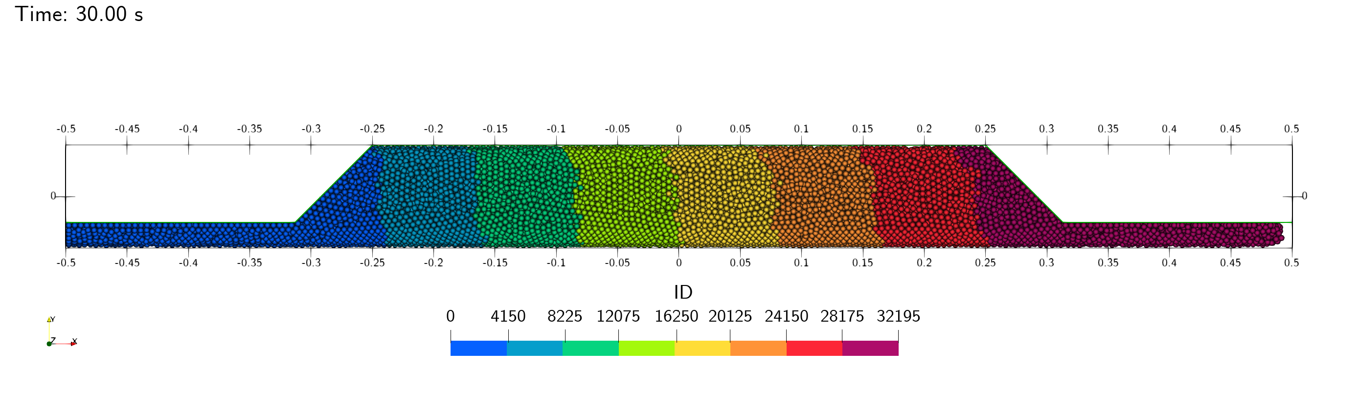
View of the pipe after the loading of particles with the insertion plane.

In summary, the simulation has three steps:

• First, we run lethe-particles loading-particles.prm to load the particles. The insertion of particles is done using the plane insertion method.

• Then, we run lethe-particles settling-particles.prm to reorganize the particles in the system. The gravity is changed to the y-direction and we wait for particles to settle.

• Finally, we call lethe-fluid-particles pneumatic-conveying.prm to simulate the dense pneumatic conveying.

We enable checkpointing in order to write the DEM checkpoint files in between the steps, which will be used as the starting point of the next.

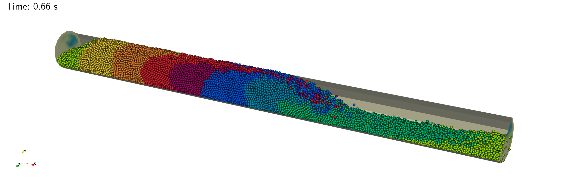
View of the pipe during the pneumatic conveying.

DEM Parameter files

Loading Particles

In this section we introduce the different sections of the parameter file loading-particles.prm.

Mesh

In this example, we simulate the transport of particles in a 1 m wide long 0.084 m diameter pipe. The conveying is processed in the x-direction through periodic boundary conditions. We use the custom cylinder of type balanced, which is prefered over the regular deal.II option for having an uniform cell size distribution in the radial direction. Cells’ size are approximately 2 times the diameter of the particles in both longitudinal and radial directions.

subsection mesh
  set type                                = cylinder
  set grid type                           = balanced
  set grid arguments                      = 45 : 0.042 : 0.5
  set initial refinement                  = 1
  set expand particle-wall contact search = true
end

Note

Note that, since the mesh is cylindrical, set expand particle-wall contact search = true. For further details, refer to DEM mesh parameters guide.

A cross-section of the resulting mesh is presented in the following figure.

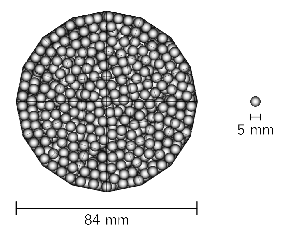
Cross-section of the mesh used in the pneumatic conveying simulation.

Lagrangian Physical Properties

The lagrangian properties were based on the work of Lavrinec et al. [1], except for the Young’s modulus that was deliberately reduced to get a higher Rayleigh critical time step.

For the particle insertion, we set gravity in x-direction to allow the packing of the particles from the right side of the pipe. The number of particles in the simulation is 32194.

Note

In order to avoid confusion with the number of particles in the parameter file, we did give the real number of particles inserted after 30 seconds. However, this is not necessary for the plane insertion method. We refer the reader to the DEM insertion info guide for further information.

subsection lagrangian physical properties
  set g                        = -9.81, 0, 0
  set number of particle types = 1
  subsection particle type 0
    set size distribution type            = uniform
    set diameter                          = 0.005
    set number of particles               = 32194
    set density particles                 = 890
    set young modulus particles           = 1e6
    set poisson ratio particles           = 0.33
    set restitution coefficient particles = 0.3
    set friction coefficient particles    = 0.3
    set rolling friction particles        = 0.2
  end
  set young modulus wall           = 1e6
  set poisson ratio wall           = 0.33
  set restitution coefficient wall = 0.3
  set friction coefficient wall    = 0.4
  set rolling friction wall        = 0.2
end

Insertion Info

As said in the previous section, the particles are inserted with the plane insertion method. The plane, in red, is located at the right-hand side of the pipe. As we can see from the following figure, the plane is positioned at an angle. Since the plane insertion method will insert one particle in a cell that is intersected by the plane, we need to place the plane so it does not intersect the area above the solid object. Particles have an initial velocity in x-direction in order to speed up the packing process and in y-direction to have more collisions and randomness in the distribution.

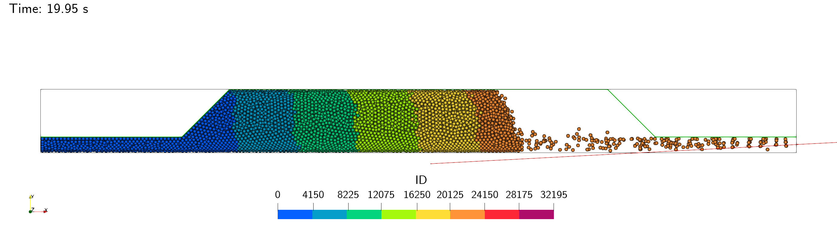
Side view of the pipe during the insertion of particles in the x-direction with the solid object (green) and the insertion plane (red).

subsection insertion info
  set insertion method              = plane
  set insertion frequency           = 400
  set insertion plane point         = 0.475, -0.0325, 0
  set insertion plane normal vector = -0.25, 4.75, 0
  set insertion maximum offset      = 0.001
  set insertion prn seed            = 19
  set initial velocity              = -0.35, 0.1, 0.0
end

Boundary Conditions DEM

Periodic boundary conditions need to be setup in the DEM simulation since we use them in the CFD-DEM simulation.

subsection DEM boundary conditions
  set number of boundary conditions = 1

  subsection boundary condition 0
    set type               = periodic
    set periodic id 0      = 1
    set periodic id 1      = 2
    set periodic direction = 0
  end
end

We need to set the periodic boundary conditions now for compatibility, but particles do not interact with these boundaries at the current stage. The next subsection explains how particles are prevented from interacting with the periodic boundaries.

Floating Walls

We use floating walls to avoid particles passing through the periodic boundary conditions. The floating walls are placed at the left and right side of the pipe. We need this pair of walls because periodic particles do not interact with the periodic boundaries.

 subsection floating walls
 set number of floating walls = 2
 subsection wall 0
   subsection point on wall
     set x = -0.5
     set y = 0
     set z = 0
   end
   subsection normal vector
     set nx = 1
     set ny = 0
     set nz = 0
   end
   set start time = 0
   set end time   = 30
 end
 subsection wall 1
   subsection point on wall
     set x = 0.5
     set y = 0
     set z = 0
   end
   subsection normal vector
     set nx = -1
     set ny = 0
     set nz = 0
   end
   set start time = 0
   set end time   = 30
 end
end

Solid Objects

The solid object is a simplex surface mesh that represents the shape of a slug. The mesh is generated with Gmsh. The following figure shows the different parts of the slug. The length of the slug core (where particles fully obstruct the pipe; in green) is 0.5 m, and 45° planes inclined are placed the rear and the front of the slug (in blue). The stationary layer (the layer between periodic slugs; in red) has a height of 0.021 m which represents 20 % of the cross-section area of the pipe.

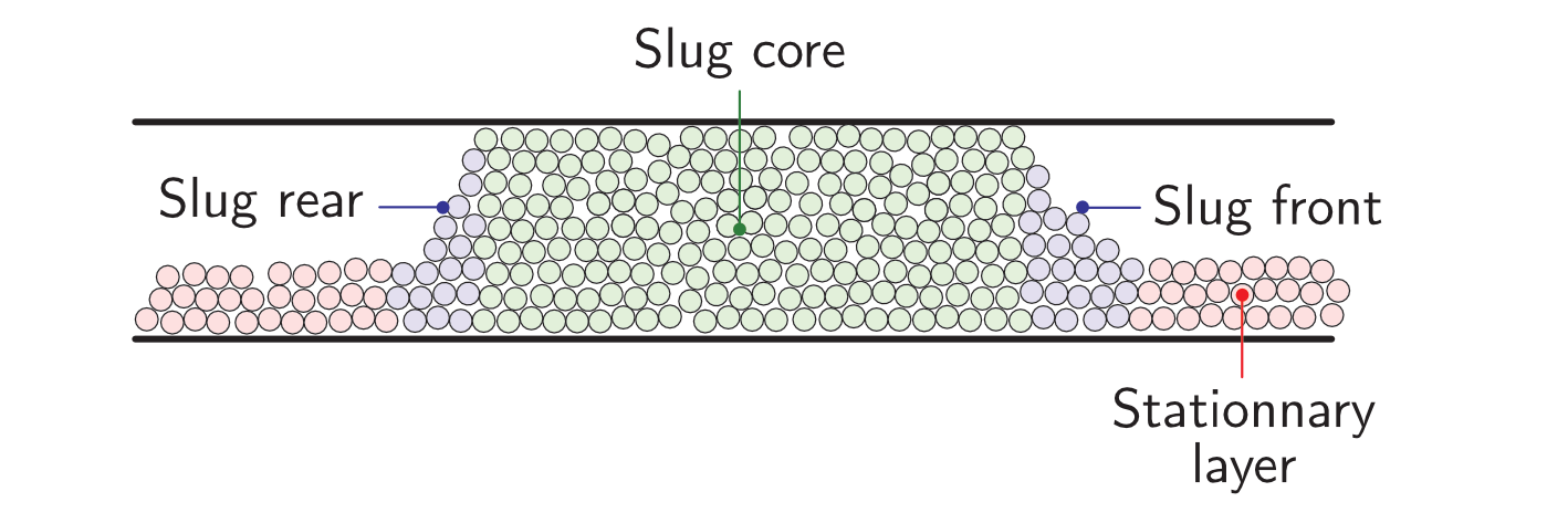
Different parts of the slug in a dense pneumatic conveying.

subsection solid objects
  set number of solids = 1
  subsection solid object 0
    subsection mesh
      set type      = gmsh
      set file name = slug-shape.msh
      set simplex   = true
    end
  end
end

Model Parameters

The model parameters are quite standard for a DEM simulation with the non-linear Hertz-Mindlin contact force model, a constant rolling resistance torque, and the velocity Verlet integration method.

Note

Here, we use the Adaptive Sparse Contacts (ASC) method to speedup the simulation,. The method will disable the contact computation in quasi-static areas which represents a significant part of the domain during the loading of the particles. Weight factor parameters for the ASC status are used in the load balancing method. The discharge plate example is a good example of the use of the ASC method with DEM.

subsection model parameters
  subsection contact detection
    set contact detection method = dynamic
    set neighborhood threshold   = 1.3
  end
  subsection load balancing
    set load balance method     = dynamic_with_sparse_contacts
    set threshold               = 0.5
    set dynamic check frequency = 8000
    set active weight factor    = 0.8
    set inactive weight factor  = 0.6
  end
  set particle particle contact force method = hertz_mindlin_limit_overlap
  set particle wall contact force method     = nonlinear
  set integration method                     = velocity_verlet
  set rolling resistance torque method       = constant_resistance
  subsection adaptive sparse contacts
    set enable adaptive sparse contacts = true
    set enable particle advection       = false
    set granular temperature threshold  = 1e-4
    set solid fraction threshold        = 0.4
  end
end

Simulation Control

Here, we define the time step and the simulation end time. 30 seconds of simulation are needed to load the particles. The long simulation time is due to the plane insertion method, which only allows for about 1000 particles per second of simulation.

subsection simulation control
  set time step        = 5e-5
  set time end         = 30
  set log frequency    = 500
  set output frequency = 1200
  set output path      = ./output_dem/
end

Restart

Checkpointing is enabled since we need the output to rerun the DEM solver to settle the particles in the pipe. The checkpointing occurs each 1.5 seconds, in case we need to stop and restart the loading simulation.

subsection restart
  set checkpoint = true
  set frequency  = 30000
  set restart    = false
  set filename   = dem
end

Settling Particles

In this section we show the difference in the parameter file settling-particles.prm needed to settle the particles with the same gravity vector as the pneumatic conveying simulation. Consequently, many sections related to the loading are not needed such as the the insertion info, the floating walls, and the solid objects.

Simulation Control

Here we allow a 2.5 seconds for the settling of the particles. Since this simulation is a restart of the loading particle simulation, the end time is 32.5 seconds.

subsection simulation control
  set time step        = 5e-5
  set time end         = 32.5
  set log frequency    = 500
  set output frequency = 1200
  set output path      = ./output_dem/
end

Restart

This simulation restarts from the previous step. Also, the checkpointing is reduced to 0.5 seconds.

subsection restart
  set checkpoint = true
  set frequency  = 10000
  set restart    = true
  set filename   = dem
end

Lagrangian Physical Properties

The main difference between the insertion and settling simulations is the direction of the gravity, which is changed to y-direction to be coherent with the next simulation using the CFD-DEM solver.

subsection lagrangian physical properties
  set g                        = 0, -9.81, 0
  set number of particle types = 1
  subsection particle type 0
    set size distribution type            = uniform
    set diameter                          = 0.005
    set number of particles               = 32194
    set density particles                 = 890
    set young modulus particles           = 1e6
    set poisson ratio particles           = 0.33
    set restitution coefficient particles = 0.3
    set friction coefficient particles    = 0.3
    set rolling friction particles        = 0.2
  end
  set young modulus wall           = 1e6
  set poisson ratio wall           = 0.33
  set restitution coefficient wall = 0.3
  set friction coefficient wall    = 0.4
  set rolling friction wall        = 0.2
end

CFD-DEM Parameter file

Pneumatic Conveying Simulation

The CFD simulation is carried out using the slug generated in the previous step. We will discuss the different sections of the parameter file used for the CFD-DEM simulation. The mesh and the DEM boundary condition sections are identical to the ones in the DEM simulations and will not be shown again.

Lagrangian Physical Properties

The physical properties of the particles are the same as in the DEM simulations, except for the Young’s modulus that was increased to use the same value as the article [1].

subsection lagrangian physical properties
  set g                        = 0, -9.81, 0
  set number of particle types = 1
  subsection particle type 0
    set size distribution type            = uniform
    set diameter                          = 0.005
    set number of particles               = 32194
    set density particles                 = 890
    set young modulus particles           = 1e7
    set poisson ratio particles           = 0.33
    set restitution coefficient particles = 0.3
    set friction coefficient particles    = 0.3
    set rolling friction particles        = 0.2
  end
  set young modulus wall           = 1e7
  set poisson ratio wall           = 0.33
  set restitution coefficient wall = 0.3
  set friction coefficient wall    = 0.4
  set rolling friction wall        = 0.2
end

Model Parameters

Model parameters are the same as in the DEM simulation, but without load balancing or adaptive sparse contacts.

subsection model parameters
  subsection contact detection
    set contact detection method = dynamic
    set neighborhood threshold   = 1.3
  end
  set particle particle contact force method = hertz_mindlin_limit_overlap
  set particle wall contact force method     = nonlinear
  set integration method                     = velocity_verlet
  set rolling resistance torque method       = constant_resistance
end

Simulation Control

The simulation lasts 5 seconds and the CFD time step is 5e-4 seconds.

subsection simulation control
  set method               = bdf1
  set output name          = cfd_dem
  set output frequency     = 10
  set time end             = 5
  set time step            = 5e-4
  set output path          = ./output/
end

Physical Properties

The physical properties of air are the same as Lavrinec et al. [1].

subsection physical properties
  subsection fluid 0
    set kinematic viscosity = 1.5e-5
    set density             = 1.205
  end
end

Boundary Conditions

The boundary condition at the wall of the pipe is a weak function where the Dirichlet condition is weakly imposed as a no-slip condition. The inlet and the outlet have periodic boundaries. See here for more information on boundary conditions.

subsection boundary conditions
  set number = 2
  subsection bc 0
    set id   = 0
    set type = function weak
    set beta = 100
    subsection u
      set Function expression = 0
    end
    subsection v
      set Function expression = 0
    end
    subsection w
      set Function expression = 0
    end
  end
  subsection bc 1
    set id                 = 1
    set type               = periodic
    set periodic_id        = 2
    set periodic_direction = 0
  end
end

Flow control

Since the simulation has periodic boundary conditions, a correction volumetric force is needed to drive the flow to compensate the pressure drop in the pipe. For this, we use the dynamic flow controller. Here, we also apply a proportional force on particles. The average velocity is set to 3 m/s, this correspond to the average over the entire domain considering the void fraction. The flow controller performs well for CFD simulation, but needs some tuned for CFD-DEM simulation.

By default, the controller has a high stiffness and aims to correct the flow in the next time step. However, the carrying of particles by the flow leads to a response time that is not taken into account and results in a oscillation of the velocity of the flow. To avoid this, we use the volumetric force threshold beta threshold and the alpha relaxation parameter. Here, the volumetric force value will not be updated if the new value is within the 5% of the previous value. Also, the correction to apply to the previous volumetric force value is reduced by a factor of 0.25. This way, the velocity of the flow and the particles are more stable.

subsection flow control
  set enable               = true
  set enable beta particle = true
  set average velocity     = 3
  set flow direction       = 0
  set beta threshold       = 0.05
  set alpha                = 0.25
  set verbosity            = verbose
end

Void Fraction

We choose the quadrature centred method (QCM) to calculate the void fraction. The l2 smoothing factor we choose is the square of twice the diameter of the particles.

subsection void fraction
  set mode                = qcm
  set read dem            = true
  set dem file name       = dem
  set l2 smoothing factor = 0.0001
end

CFD-DEM

We use the Di Felice drag model, the Saffman lift force, the buoyancy force, and the pressure force. The coupling frequency is set to 100, which means that the DEM time step is 5e-6 s. The DEM time step is 3.5% of the Rayleigh critical time step. The grad-div stabilization is used with a length scale of 0.084, the diameter of the pipe.

subsection cfd-dem
  set grad div               = true
  set drag model             = difelice
  set saffman lift force     = true
  set buoyancy force         = true
  set pressure force         = true
  set coupling frequency     = 100
  set implicit stabilization = false
  set grad-div length scale  = 0.084
  set particle statistics    = true
end

Non-linear Solver

We use the inexact Newton non-linear solver to minimize the number of time the matrix of the system is assembled. This is used to increase the speed of the simulation, since the matrix assembly requires significant computations.

subsection non-linear solver
  subsection fluid dynamics
    set solver           = inexact_newton
    set matrix tolerance = 0.1
    set reuse matrix     = true
    set tolerance        = 1e-4
    set max iterations   = 10
    set verbosity        = quiet
  end
end

Running the Simulations

Launching the simulations is as simple as specifying the executable name and the parameter file. Assuming that the lethe-particles and lethe-fluid-particles executables are within your path, the simulations can be launched in parallel as follows:

mpirun -np 8 lethe-particles loading-particles.prm

mpirun -np 8 lethe-particles settling-particles.prm

Note

Running the particle loading simulation using 8 cores takes approximately 30 minutes and the particle settling simulation takes approximately 1 minute.

Once the previous programs have finished running, you can finally launch the pneumatic conveying simulation and get the simulation log for post-processing with the following command:

mpirun -np 8 lethe-fluid-particles pneumatic-conveying.prm | tee pneumatic-log.out

Note

Running the pneumatics conveying simulation using 8 cores takes approximately 2.25 hours. Running all the executables in sequence will take less than 3 hours.

Lethe will generate a number of files. The most important one bears the extension .pvd. It can be read by popular visualization programs such as Paraview.

Results

The particle loading and settling simulation should look like this:

The pneumatic conveying simulation should look like this:

Note

The pneumatic conveying simulation lasts 5 seconds in this example, but last 10 seconds in the video. You can change the end time in the parameter file.

Post-processing

The data is extracted with the Lethe PyVista tool and post-processed with custom functions in the files pyvista_utilities.py and log_utilities.py. Extraction, post-processing and plotting are automated in the script pneumatic-conveying_post-processing.py:

python3 pneumatic-conveying_post-processing.py

The script will generate the figure and print the results in the console. If you want to modify the path or the filenames, you have to modify the script.

Mass Flow Rate and Velocities

Here we show the average velocities for the fluid, the slug and the particles in slug. The beta force, the averaged solid mass flow rate and the slug length over time are also shown. The shaded area represents the transient state. The quasi-steady state is approximated when velocities fluctuate around the same values.

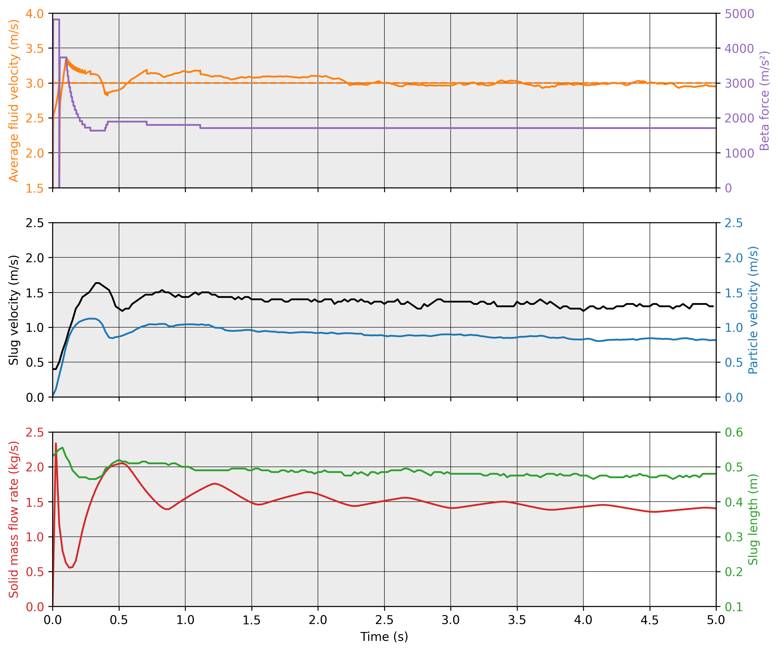
Results of the pneumatic conveying simulation.

The time-averaged values of velocities at quasi-steady state are shown in the following table.

Time-averaged velocities at quasi-steady state.

	Fluid	Slug	Particles
Velocity (m/s)	2.98	1.30	0.83
Standard deviation (m/s)	0.02	0.02	0.01

According to Lavrinec et al. [2], the average slug velocity has a linear relationship with the particle in slug velocity and the diameter of the pipe such as:

\[\bar{u}_{\mathrm{slug}} = 0.967 \bar{u}_{\mathrm{particles}} + 0.5\sqrt{gD}\]

From this formula, the calculated slug velocity is 1.25 m/s. Considering that this case was simplified for the sake of the example, that the data in quasi-steady state is not computed for a long simulation time (1 s), and especially considering the standard deviation of the results, this value is considered satisfactory.

The time-averaged solid mass flow rate is 1.40 kg/s (no standard deviation are given since the instant mass flow rate always fluctuates) and the length of the slug is 0.47 ± 0.01 m.

References

[1] (1,2,3,4)

A. Lavrinec, O. Orozovic, H. Rajabnia, K. Williams, M. Jones & G. Klinzing, “An assessment of steady-state conditions in single slug horizontal pneumatic conveying.” Particuology, vol. 58, pp. 187-195, 2021. doi: 10.1016/j.partic.2021.04.007.

[2]

A. Lavrinec, O. Orozovic, H. Rajabnia, K. Williams, M. Jones et G. Klinzing, “Velocity and porosity relationships within dense phase pneumatic conveying as studied using coupled CFD-DEM.” Powder Technology, vol. 375, pp. 89–100, 2020. doi: 10.1016/j.powtec.2020.07.070.