Liquid-Solid Fluidized Bed

It is strongly recommended to visit DEM parameters and CFD-DEM parameters for more detailed information on the concepts and physical meaning of the parameters ind DEM and CFD-DEM.

Features

• Solvers: lethe-particles and lethe-fluid-particles

• Three-dimensional problem

• Displays the selection of models and physical properties

• Simulates a solid-liquid fluidized bed

• Postprocessing code available

Files Used in This Example

All files mentioned below are located in the example’s folder (examples/unresolved-cfd-dem/liquid-solid-fluidized-bed).

• Parameter file of particles generation and packing: packing-particles.prm

• Parameter file for CFD-DEM simulation of the liquid-solid fluidized bed: liquid-solid-fluidized-bed.prm

• Postprocessing Python script: lsfb_postprocessing.py

Description of the Case

This example simulates the fluidization of spherical particles in water. It is meant to reproduce the behavior observed experimentally in a pilot-scale equipment with the same characteristics as the simulations.

We use two different types of particles [1]: alginate \((d_p = 2.66 \: \text{mm}\), \(\rho_p = 1029 \: \text{kg} \cdot \text{m}^{-3})\) and alumina \((d_p = 3.09 \: \text{mm}\), \(\rho_p = 3586 \: \text{kg} \cdot \text{m}^{-3})\).

A representation of this equipment is shown. The fluidization region comprises a \(1.0 \: \text{m}\) height, \(10 \: \text{cm}\) diameter cylinder made of acrylic. More details about the experimental setup can be found in Ferreira et al. [1] and Ferreira et al [2].

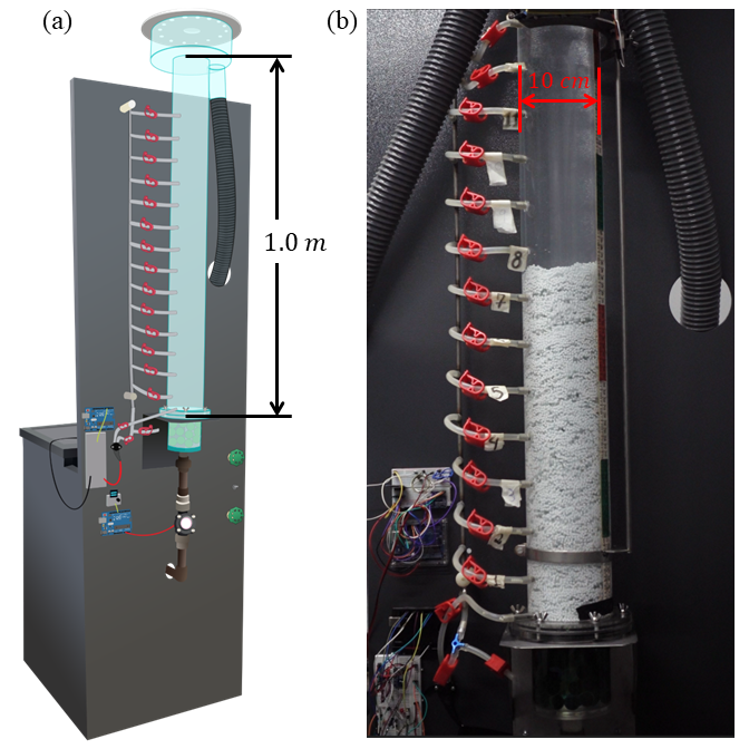
Pilot-scale fluidized bed used as reference for simulations in this example. Image includes (a) schematic representation of the bed and (b) picture of the equipment in operation. Adapted from Ferreira et al [1].

DEM Parameter File

As in the other examples of this documentation, we use Lethe-DEM to fill the bed with particles. We enable check-pointing in order to write the DEM checkpoint files which will be used as the starting point of the CFD-DEM simulation. Then, we use the lethe-fluid-particles solver within Lethe to simulate the fluidization of the particles by initially reading the checkpoint files from the DEM simulation.

All parameter subsections are described in the Parameters section of the documentation.

To set-up the cylinder fluidized bed case, we first fill the bed with particles.

We first introduce the different sections of the parameter file packing-particles.prm needed to run this simulation.

Mesh

In this example, we are simulating a cylindrical fluidized bed that has a half length of \(0.55 \: \text{m}\) (\(10 \: \text{cm}\) higher than the fluidization region in the experimental setup), and a diameter of \(10 \: \text{cm}\). We use the subdivided_cylinder GridGenerator in order to generate the mesh. The cylindrical bed is divided \(132 \: \text{times}\) in the \(x\) direction (height) and \(12 \: \text{times}\) in \(y\) and \(z\) directions (\(6 \: \text{times}\) along the radius). The following portion of the DEM parameter file shows the function called:

subsection mesh
  set type               = dealii
  set grid type          = subdivided_cylinder
  set grid arguments     = 33:0.05:0.55
  set initial refinement = 2
  set expand particle-wall contact search = true
end

Note

Note that, since the mesh is cylindrical, set expand particle-wall contact search = true. Details on this in the DEM mesh parameters guide.

A cross-section of the resulting mesh is presented in the following figure.

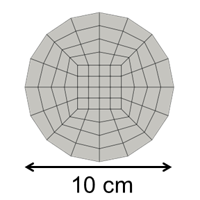
Cross-section of the mesh used in liquid-solid fluidized bed simulations.

Floating Walls

A floating wall is added \(10 \: \text{cm}\) above the bottom of the mesh, so that void fraction discontinuities can be avoided. The remaining region above the floating wall is \(1 \: \text{m}\) high, as in the experimental setup.

subsection floating walls
  set number of floating walls = 1
  subsection wall 0
    subsection point on wall
      set x = -0.45
      set y = 0
      set z = 0
    end
    subsection normal vector
      set nx = 1
      set ny = 0
      set nz = 0
    end
    set start time = 0
    set end time   = 50
  end
end

Note

Note that end time is higher than time end in simulation control, so that the floating wall remains for the whole simulation.

Simulation Control

Here, we define the time-step and the simulation end time.

subsection simulation control
  set time step        = 0.000005
  set time end         = 2.5
  set log frequency    = 20000
  set output frequency = 20000
  set output path      = ./output_dem/
end

Important

It is important to define the time end to include the time required to insert the particles and the time the it takes for particles to settle.

Restart

The lethe-fluid-particles solver requires reading several DEM files to start the simulation. For this, we have to write the DEM simulation information. This is done by enabling the check-pointing option in the restart subsection. We give the written files a prefix “dem” set in the set filename option. The DEM parameter file is initialized exactly as the cylindrical packed bed example. The difference is in the number of particles, their physical properties, and the insertion box defined based on the new geometry. For more explanation about the individual subsections, refer to the DEM parameters and the CFD-DEM parameters.

subsection restart
  set checkpoint = true
  set frequency  = 20000
  set restart    = false
  set filename   = dem
end

Model Parameters

The subsection on model parameters is explained in the DEM model parameters guide and DEM examples.

subsection model parameters
  subsection contact detection
    set contact detection method = dynamic
    set neighborhood threshold   = 1.5
  end
  subsection load balancing
    set load balance method     = dynamic
    set threshold               = 0.5
    set dynamic check frequency = 10000
  end
  set particle particle contact force method = hertz_mindlin_limit_overlap
  set particle wall contact force method     = nonlinear
  set integration method                     = velocity_verlet
end

Lagrangian Physical Properties

The lagrangian properties were taken from Ferreira et al [1].

subsection lagrangian physical properties
  set g                        = -9.81, 0, 0
  set number of particle types = 1
  subsection particle type 0
    set size distribution type            = uniform
    set diameter                          = 0.003087
    set number                            = 72400
    set density particles                 = 3585.9
    set young modulus particles           = 1e7
    set poisson ratio particles           = 0.3
    set restitution coefficient particles = 0.9
    set friction coefficient particles    = 0.1
    set rolling friction particles        = 0.2
  end
  set young modulus wall           = 1e7
  set poisson ratio wall           = 0.3
  set restitution coefficient wall = 0.2
  set friction coefficient wall    = 0.1
  set rolling friction wall        = 0.3
end

The number of particles used for alginate particles is \(107\;\! 960\).

Insertion Info

The volume of the insertion box should be large enough to fit all particles. Also, its bounds should be located within the mesh generated in the Mesh subsection.

subsection insertion info
  set insertion method                               = volume
  set inserted number of particles at each time step = 48841 # for alginate, we recommend 79600
  set insertion frequency                            = 200000
  set insertion box points coordinates               = -0.15, -0.035, -0.035 : 0.53, 0.035, 0.035
  set insertion distance threshold                   = 1.3
  set insertion maximum offset                       = 0.3
  set insertion prn seed                             = 19
end

Note

Particles need to be fully settled before the fluid injection. Hence, time end in subsection simulation control needs to be chosen accordingly.

Running the DEM Simulation

Launching the simulation is as simple as specifying the executable name and the parameter file. Assuming that the lethe-particles executable is within your path, the simulation can be launched in parallel as follows:

mpirun -np 8 lethe-particles packing-particles.prm

Lethe will generate a number of files. The most important one bears the extension .pvd. It can be read by popular visualization programs such as Paraview.

Note

Running the packing of alumina particles should take approximately \(57 \: \text{minutes}\) on \(16 \: \text{cores}\). For the alginate particles, it takes approximately \(1 \: \text{hour}\) and \(53 \: \text{minutes}\).

Now that the particles have been packed inside the cylinder, it is possible to simulate the fluidization of particles.

CFD-DEM Parameter File

The CFD simulation is to be carried out using the packed bed simulated in the previous step. We will discuss the different parameter file sections. The mesh section is identical to that of the DEM so it will not be shown again.

Simulation Control

The long simulation is due to the small difference between particles and liquid densities, meaning that it takes very long to reach the pseudo-steady state.

subsection simulation control
  set method            = bdf1
  set output name       = cfd_dem
  set output frequency  = 100
  set time end          = 20
  set time step         = 0.001
  set output path       = ./output/
end

Since the alumina particles are more than \(3 \: \text{times}\) denser than alginate particles, the pseudo-steady state is reached after very different times (according to Ferreira et al [1]. \(4\) and \(10 \: \text{seconds}\) of real time, respectively). Because of this, we use set time end = 35 for the alginate.

Physical Properties

The physical properties subsection allows us to determine the density and viscosity of the fluid. The values are meant to reproduce the characteristics of water at \(30 \: \text{°C}\).

subsection physical properties
  subsection fluid 0
    set kinematic viscosity = 0.0000008379
    set density             = 997
  end
end

Initial Conditions

For the initial conditions, we choose zero initial conditions for the velocity.

subsection initial conditions
  set type = nodal
  subsection uvwp
      set Function expression = 0; 0; 0; 0
  end
end

Boundary Conditions

For the boundary conditions, we choose a slip boundary condition on the walls (id = 0) and an inlet velocity of \(0.157\;\! 033 \: \text{m/s}\) at the lower face of the bed (id = 1).

subsection boundary conditions
  set number = 2
  subsection bc 0
    set id   = 0
    set type = slip
  end
  subsection bc 1
    set id   = 1
    set type = function
    subsection u
      set Function expression = 0.157033
    end
    subsection v
      set Function expression = 0
    end
    subsection w
      set Function expression = 0
    end
  end
end

The following sections for the CFD-DEM simulations are the void fraction subsection and the CFD-DEM subsection. These subsections are described in detail in the CFD-DEM parameters .

Void Fraction

We choose the particle centroid method (PCM) to calculate void fraction. The l2 smoothing factor we choose is around the square of twice the particle’s diameter, as in the other examples.

subsection void fraction
  set mode                = pcm
  set read dem            = true
  set dem file name       = dem
  set l2 smoothing factor = 2.8387584e-5
end

Note

Note that void fraction is not bound in this case. The size of the particles used in this example forces us to use a very coarse mesh. Bounding void fraction would lead to instability in the present case.

CFD-DEM

Different from gas-solid fluidized beds, buoyancy, pressure force, shear stress are not negligible. All these forces are considered in this example.

Saffman lift force is proven to be very important to properly reproduce particles’ dynamics in the liquid-fluidized bed [1].

subsection cfd-dem
  set vans model         = modelA
  set grad div           = true
  set drag model         = rong
  set buoyancy force     = true
  set shear force        = true
  set pressure force     = true
  set saffman lift force = true
  set coupling frequency = 100
  set void fraction time derivative = false
end

Warning

Void-fraction time-derivative lead to significant instability in the case of liquid-fluidized beds, hence we do not use it.

Non-linear Solver

We use the inexact Newton non-linear solver to minimize the number of time the matrix of the system is assembled. This is used to increase the speed of the simulation, since the matrix assembly requires significant computations.

subsection non-linear solver
  subsection fluid dynamics
    set solver           = inexact_newton
    set tolerance        = 1e-10
    set max iterations   = 10
    set verbosity        = verbose
  end
end

Linear Solver

subsection linear solver
  subsection fluid dynamics
    set method                                = gmres
    set max iters                             = 5000
    set relative residual                     = 1e-3
    set minimum residual                      = 1e-11
    set preconditioner                        = ilu
    set ilu preconditioner fill               = 1
    set ilu preconditioner absolute tolerance = 1e-14
    set ilu preconditioner relative tolerance = 1.00
    set verbosity                             = verbose
  end
end

Running the CFD-DEM Simulation

The simulation is run (on \(8 \: \text{cores}\)) using the lethe-fluid-particles application as follows:

mpirun -np 8 lethe-fluid-particles liquid-solid-fluidized-bed.prm

The \(20\)-second simulations with alumina took approximately \(24 \: \text{hours}\) and \(30 \: \text{minutes}\) on \(16 \: \text{cores}\) and \(8 \: \text{hours}\) and \(44 \: \text{minutes}\) on \(32 \: \text{cores}\).

The \(35\)-second simulations with alginate particles took about \(28 \: \text{hours}\) on \(16 \: \text{cores}\).

Results

We briefly comment on some results that can be extracted from this example.

Important

This example includes a postprocessing file written in Python that uses the lethe_pyvista_tools. module.

Important

To use the code, run python3 lsfb_postprocessing.py $PATH_TO_YOUR_CASE_FOLDER. The code will generate several graphics showing the pressure profile within the bed, which are going to be stored in $PATH_TO_YOUR_CASE_FOLDER/P_x. It will also generate a deltaP_t.csv file with the total pressure difference for each time-step. Additionally, it generates a void fraction as a function of time graphic (eps_t.png).

Important

You need to ensure that the lethe_pyvista_tools is working on your machine. Click here for details.

Side View

Here we show comparison between the experimentally observed and simulated behavior of the liquid-solid fluidized bed with alumina.

The void fraction and velocity profile of the fluid are also shown.

Total Pressure Drop and Bed Expansion

In fluidized beds, the total pressure drop (\(- \Delta p\)) reflects the total weight of particles (\(M\)). The following equation is derived from a force balance inside the fluidized bed [3].

\[H(1 - \bar{\varepsilon}_f) = \frac{- \Delta p}{(\rho_p - \rho_f)g} = \frac{M}{\rho_p A} = \mathrm{constant}\]

where \(H\) is the total bed height, \(\bar{\varepsilon}_f\) is the average fluid fraction (void fraction) at the bed region, \(\rho_p\) and \(\rho_f\) are the densities of the particles and the fluid (respectively), and \(A\) is the cross-section area of the equipment.

Liquid fluidized beds are very uniform in terms of particles distribution, resulting in an uniform distribution of \(\varepsilon_f\) along the be height. From this hypothesis, we can conclude that, for a constant and uniform fluid inlet flow rate, the pressure slope is:

\[\left.- \frac{\mathrm{d} p }{\mathrm{d} z}\right|_{z = 0}^{z = H} \approx \mathrm{constant}\]

With the pressure slope, it is also possible to determine the bed void fraction manipulating the first equation, which gives:

\[\bar{\varepsilon}_f = 1 - \frac{\left.- \frac{\mathrm{d} p }{\mathrm{d} z}\right|_{z = 0}^{z = H} }{(\rho_p - \rho_f)g}\]

The resulting behavior of the pressure along the bed height and the void fraction with time is shown in the following animation.

Particles Dynamics

Since the fluidization occurs in a high density fluid, the density difference between alginate and alumina particles have a significant impact on the velocity of the particles inside the bed.

The following animation is in real time. It is possible to notice that, for a similar bed height, the bed of alumina particles expands way faster than the alginate.

References

[1] (1,2,3,4,5,6)

V. O. Ferreira, T. E. Geitani, D. Silva, B. Blais, and G. C. Lopes, “In-depth validation of unresolved CFD-DEM simulations of liquid fluidized beds,” Powder Technol., vol. 426, pp. 118652, Aug. 2023, doi: 10.1016/j.powtec.2023.118652.

[2]

V. O. Ferreira, D. Silva Junior, K. R. B. de Melo, B. Blais, and G. C. Lopes, “Prediction of the bed expansion of a liquid fluidized bed bioreactor applied to wastewater treatment and biogas production,” Energy Convers. Manag., vol. 290, pp. 117224, Aug. 2023, doi: 10.1016/j.enconman.2023.117224.

[3]

W.-C. Yang, Ed., Handbook of Fluidization and Fluid-Particle Systems, 1st ed. Boca Raton: CRC Press, 2003. doi: 10.1201/9780203912744.