Gas-Solid Fluidized Cylinder Bed

This example simulates the fluidization of particles in air within a cylindrical bed. It is based on the fluidized bed test case presented in the work of El Geitani et al [1] and was used to validate one of the earliest CFD-DEM implementations in Lethe. Most importantly, this example compares the pressure drop across the bed as a function of the superficial gas velocity with correlations available in the literature.

Features

• Solvers: lethe-particles, lethe-fluid-particles and lethe-fluid-particles-matrix-free, with Q1-Q1

• Three-dimensional problem

• Displays the selection of models and physical properties

• Shows the three coupling strategies for the drag force (implicit, semi-implicit and explicit)

• Simulates a cylindrical solid-gas fluidized bed

Files Used in This Example

All files mentioned below are located in the example’s folder (examples/unresolved-cfd-dem/gas-solid-fluidized-cylinder-bed).

• Parameter file for particle generation and packing: packing-particles.prm

• Parameter files for CFD-DEM simulation of the gas-solid fluidized bed: mb-fluidized-bed-modelA-pcm-explicit.prm, mb-fluidized-bed-modelA-pcm-implicit.prm, mb-fluidized-bed-modelA-pcm-semi-implicit.prm, mb-fluidized-bed-modelA-qcm-explicit.prm, mb-fluidized-bed-modelA-qcm-implicit.prm, mb-fluidized-bed-modelA-qcm-semi-implicit.prm, mf-fluidized-bed-modelA-qcm-explicit.prm, mf-fluidized-bed-modelA-qcm-implicit.prm, mf-fluidized-bed-modelA-qcm-semi-implicit.prm

• Post-processing Python script: plot-pressure.py

Description of the Case

This example simulates a gas–solid fluidized bed inside a cylindrical column (diameter \(0.02\) m, height \(0.4\) m). First, lethe-particles is used with packing-particles.prm to generate and pack spherical particles (diameter \(0.0005\) m, density \(1000\;\text{kg}/\text{m}^3\)) inside the column. After packing, the solid–fluid mixture is simulated using the model A of the VANS equations with two solvers:

1. The matrix-based CFD–DEM solver lethe-fluid-particles

   The VANS model A using the matrix-based solver is tested with two different projection filters:

   • a cell-based filter (corresponding to the Particle Centroid Method, PCM)

   • the Quadrature-Centered Method (QCM) filter.

2. The matrix-free solver lethe-fluid-particle-matrix-free

   This solver only works with the QCM filter

For more details on the different filtering approaches used in Lethe, the reader is invited to consult the Unresolved CFD-DEM section of Lethe’s theory guide. It is worth noting that in this example, the same filter is applied to both the void fraction and the particle–fluid forces, which is mathematically consistent. However, different filters can be applied to the void fraction and to the particle–fluid forces independently, if desired. Each case is run with three different coupling approaches for the drag force: explicit, implicit, and semi-implicit.

The superficial gas velocity at the inlet is varied from \(0.02\) to \(0.3\;\text{m}/\text{s}\) and the pressure drop across the bed is recorded. Results are compared with correlations from the literature for validation.

DEM Parameter File

A DEM simulation is first run to insert the particles. The subsections in the DEM parameter file packing-particles.prm that are pertinent to this example are described below.

Mesh

The particles are packed inside a cylindrical column. For this reason, the mesh type is set to cylinder with a balanced grid. This mesh uses the same input arguments as the GridGenerator::subdivided_cylinder function of Deal.II, yet leads to more uniform cells across the domain. An initial refinement level of \(2\) provides enough cells for the CFD solver while keeping the smallest cell size larger than the particle diameter. Finally, the particle–wall contact search expansion is enabled to ensure proper detection of particle–wall interactions in the curved convex geometry.

subsection mesh
    set type                                = cylinder
    set grid type                           = balanced
    set grid arguments                      = 44:0.01:0.22
    set initial refinement                  = 2
    set expand particle-wall contact search = true
end

Simulation Control

The simulation control subsection specifies the time step, time end, log frequency, output frequency and output path of the DEM simulation. output boundaries is set to true so that the cylindrical column walls are also written to file for visualization. The time step corresponds to approximately \(11\%\) of the Rayleigh timestep, ensuring numerical stability. The simulation end time is set to \(0.7\) s, a duration sufficient for all inserted particles to settle within the column.

subsection simulation control
    set time step         = 0.000005
    set time end          = 0.7
    set log frequency     = 1000
    set output frequency  = 2000
    set output path       = ./output_dem/
    set output boundaries = true
end

Restart

The initial state of the particles in the CFD-DEM solver corresponds to the final state of the DEM packing simulation. Therefore, the restart subsection is used to enable writing the checkpoint files that need to be read by the CFD-DEM solver. The prefix of these files in set as dem in the filename option.

subsection restart
    set checkpoint = true
    set frequency  = 10000
    set restart    = false
    set filename   = dem
end

Model Parameters

Details on the model parameters subsection are provided in the DEM Model Parameters guide and other DEM examples. The neighborhood threshold is set to \(1.1\) as an adequate compromise between the number of contact detection steps and the number of neighbours of each particle. This is mostly for computational efficiency and a value of \(1.2\) or \(1.3\) could also be used here.

subsection model parameters
    subsection contact detection
        set contact detection method = dynamic
        set neighborhood threshold   = 1.1
    end
    subsection load balancing
        set load balance method = frequent
        set frequency           = 10000
    end
    set particle particle contact force method = hertz_mindlin_limit_overlap
    set particle wall contact force method     = nonlinear
    set integration method                     = velocity_verlet
end

Lagrangian Physical Properties

The lagrangian physical properties subsection defines the physical properties of the particles and walls in the simulation. All properties are chosen to match those used in the work of El Geitani et al [1]. Accordingly, the cylindrical bed is filled with \(200\;000\) particles, each with a diameter of \(500\;\mu\text{m}\) and a density of \(1000\;\text{kg}/\text{m}^3\).

subsection lagrangian physical properties
    set g                        = -9.81, 0, 0
    set number of particle types = 1
    subsection particle type 0
        set size distribution type            = uniform
        set diameter                          = 0.0005
        set number of particles               = 200000
        set density particles                 = 1000
        set young modulus particles           = 1e6
        set poisson ratio particles           = 0.3
        set restitution coefficient particles = 0.9
        set friction coefficient particles    = 0.1
        set rolling friction particles        = 0.1
    end
    set young modulus wall           = 1e6
    set poisson ratio wall           = 0.3
    set restitution coefficient wall = 0.9
    set friction coefficient wall    = 0.1
    set rolling friction wall        = 0.1
end

Insertion Info

The particles are inserted into the cylindrical column using the insertion info subsection. All the particles are inserted at the first iteration and the insertion box dimensions are chosen so that it contains all particles.

subsection insertion info
    set insertion method                               = volume
    set inserted number of particles at each time step = 200000
    set insertion frequency                            = 200000
    set insertion box points coordinates               = -0.179, -0.0065, -0.0065 : 0.2, 0.0065, 0.0065
    set insertion distance threshold                   = 1.1
    set insertion maximum offset                       = 0.02
    set insertion prn seed                             = 19
    set insertion direction sequence                   = 1, 2, 0
end

Floating Walls

To allow the gas flow to develop before reaching the particles, the latter are packed above a floating wall located 0.04 m above the fluid inlet. This wall is defined in the floating walls subsection with a normal vector pointing in the positive x-direction.

subsection floating walls
    set number of floating walls = 1
    subsection wall 0
        set point on wall = -0.18, 0., 0.
        set normal vector = 1., 0., 0.
        set start time    = 0
        set end time      = 100
    end
end

Running the DEM Simulation

The packing simulation can be launched on 16 processors using the following command:

mpirun -np 16 lethe-particles packing-particles.prm

Note

Running this simulation should take approximately 1 hour and 10 minutes on 16 cores.

Now that the particles are packed inside the cylindrical column, the CFD-DEM simulation can be set up.

CFD-DEM Parameter File

The CFD-DEM simulation is run using the matrix-based solver lethe-fluid-particles or the matrix-free solver lethe-fluid-particles-matrix-free. For the matrix-based solver, six parameter files are provided to test VANS model A with two projection filters (cell-based and QCM) and three different drag coupling approaches (explicit, implicit, and semi-implicit). The matrix-free solver is also tested with the QCM filter and the three drag coupling schemes. The main description in this section follows the matrix-based parameter file mb-fluidized-bed-modelA-qcm-semi-implicit.prm. Differences associated with the remaining parameter files will be highlighted where relevant.

The objective of the simulations is to predict the pressure drop across the bed as a function of the Reynolds number based on the superficial gas velocity and the column diameter:

\[\mathrm{Re} = \frac{U_{\mathrm{g}} D}{\nu_{\mathrm{f}}}\]

where \(U_{\mathrm{g}}\) is the superficial gas velocity, \(D\) is the column diameter and \(\nu_{\mathrm{f}}\) is the kinematic viscosity of the fluid. For a Reynolds number interval ranging from \(200\) to \(600\), the gas inlet velocity is varied from \(0.02\;\text{m/s}\) to \(0.3\;\text{m/s}\) in increments of \(0.02\;\text{m/s}\), each value applied for \(0.05\) s.

Simulation Control

To reach an inlet velocity of \(0.3\;\text{m/s}\), the CFD-DEM simulation is run for a total time of \(0.75\) s with a time step of \(0.0002\) s. For cases with an explicit drag coupling, the time step is reduced to \(0.0001\) s to ensure numerical stability.

subsection simulation control
    set method           = bdf1
    set output frequency = 50
    set time end         = 0.75
    set time step        = 0.0002
end

Physical Properties

The gas is taken to have a density of \(1\;\text{kg/m}^3\) and a kinematic viscosity of \(10^{-5}\;\text{m}^2/\text{s}\).

subsection physical properties
    subsection fluid 0
        set kinematic viscosity = 0.00001
        set density             = 1
    end
end

Boundary Conditions

The boundary conditions are chosen as follows: a no-slip condition on the lateral wall of the column (id = 0), a time-dependent inlet velocity defined as a piecewise constant function of time with \(0.02\;\text{m/s}\) increments every \(0.05\) s (id = 1), and an outlet condition on the top wall of the column (id = 2).

subsection boundary conditions
    set number = 3
    set time dependent = true
    subsection bc 0
        set id   = 0
        set type = slip
    end
    subsection bc 1
        set id   = 1
        set type = function
        subsection u
        set Function expression = min(0.02 * floor(t / 0.05 + 1), 0.3)
        end
        subsection v
        set Function expression = 0
        end
        subsection w
        set Function expression = 0
        end
    end
    subsection bc 2
        set id   = 2
        set type = outlet
    end
end

Void Fraction

The dem file name corresponds to the files written during the previous DEM simulation using checkpointing. The calculation method is set to qcm, with the sphere’s radius chosen such that its volume equals the cell’s volume by setting qcm sphere equal cell volume to true. For cases using the PCM filter, the void fraction mode is set to pcm instead. A smoothing length equal to twice the particle diameter is used.

subsection void fraction
    set mode                         = qcm
    set qcm sphere equal cell volume = true
    set read dem                     = true
    set dem file name                = dem
    set l2 smoothing length          = 0.001
end

CFD-DEM

All hydrodynamic forces are enabled in the cfd-dem subsection. This allows testing the different models. Grad-div stabilization is also enabled to improve mass conservation, using a length-scale equal to the column’s radius, which is of the same order of the characteristic length of the flow, as recommended in the CFD-DEM parameters section. In simulations of this example using the QCM filter, the parameter project particle forces is set to true, to use the QCM filter to calculate the particle-fluid forces (by default, this parameter is false, and the cell-based filter is used to calculate the particle-fluid forces term in the VANS equations). The drag coupling parameter is set to the desired coupling approach and defaults to semi-implicit.

subsection cfd-dem
    set grad div                      = true
    set grad-div length scale         = 0.01
    set void fraction time derivative = true
    set drag force                    = true
    set buoyancy force                = true
    set shear force                   = true
    set pressure force                = true
    set drag model                    = difelice
    set coupling frequency            = 100
    set vans model                    = modelA
    set drag coupling                 = semi-implicit
    set project particle forces       = true
end

Post-processing

The pressure drop is calculated across the bed. The parameters inlet boundary id and outlet boundary id are specified as the inlet and outlet of the column, respectively.

subsection post-processing
    set calculate pressure drop = true
    set inlet boundary id       = 1
    set outlet boundary id      = 2
    set output frequency        = 1
    set verbosity               = verbose
end

Non-linear Solver

The newton nonlinear solver is used. The tolerance is selected to balance simulation time and accuracy.

subsection non-linear solver
    subsection fluid dynamics
        set solver           = newton
        set tolerance        = 1e-8
        set max iterations   = 10
        set verbosity        = verbose
    end
end

Running the CFD-DEM Simulation

The simulations are launched with the matrix-based solver (and corresponding parameter file) using the following command:

mpirun -np $numproc lethe-fluid-particles mb-fluidized-bed-modelA-qcm-semi-implicit.prm

where $numproc represents the number of processors to be used.

The matrix-free solver is run following:

mpirun -np $numproc lethe-fluid-particles-matrix-free mf-fluidized-bed-modelA-qcm-semi-implicit.prm

Note

The simulation runtimes on 128 cores, which are approximate, are as follows:

Solver	VANS Model	Force projection	Drag coupling | Simulation runtime
Matrix-based	A	PCM (Cell-based)	Explicit	2 h 50 min
Matrix-based	A	PCM (Cell-based)	Semi-implicit	1 h 9 min
Matrix-based	A	PCM (Cell-based)	Implicit	1 h 25 min
Matrix-based	A	QCM	Explicit	2 h 11 min
Matrix-based	A	QCM	Semi-implicit	1 h 5 min
Matrix-based	A	QCM	Implicit	1 h 39 min
Matrix-free	A	QCM	Explicit	1 h 56 min
Matrix-free	A	QCM	Semi-implicit	54 min
Matrix-free	A	QCM	Implicit	1 h 16 min

Results

The pressure drop is calculated during the simulation. In the post-processing Python script, for each velocity value (which lasts for \(0.05\) s), we average the pressure drop over the last \(0.025\) s and calculate the corresponding standard deviation. The resulting mean pressure drop is then plotted as a function of the Reynolds number, with the standard deviation shown as error bars. The vertical lines correspond to the fluidization limit predicted by the Wen-Yu [2] correlation:

\[\mathrm{Re}_{\text{mf}} = \left(33.7^2 + 0.0408 \, Ar \right)^{0.5} - 33.7\]

and that predicted by Noda et al [3]:

\[\mathrm{Re}_{\text{mf}} = \left(19.29^2 + 0.0276 \, Ar \right)^{0.5} - 19.29\]

Here, the subscript \(\mathrm{mf}\) refers to minimum fluidization, and \(\mathrm{Ar}\) is the Archimedes number, which depends on the acceleration due to gravity, \(g\), the fluid density, \(\rho_{\mathrm{f}}\), and dynamic viscosity, \(\mu_{\mathrm{f}}\), as well as the particle diameter, \(d_{\mathrm{p}}\), and particle density, \(\rho_{\mathrm{p}}\):

\[\mathrm{Ar} = \frac{g \rho_{\mathrm{f}} (\rho_{\mathrm{p}} - \rho_{\mathrm{f}}) d_{\mathrm{p}}^3}{\mu_{\mathrm{f}}^2}.\]

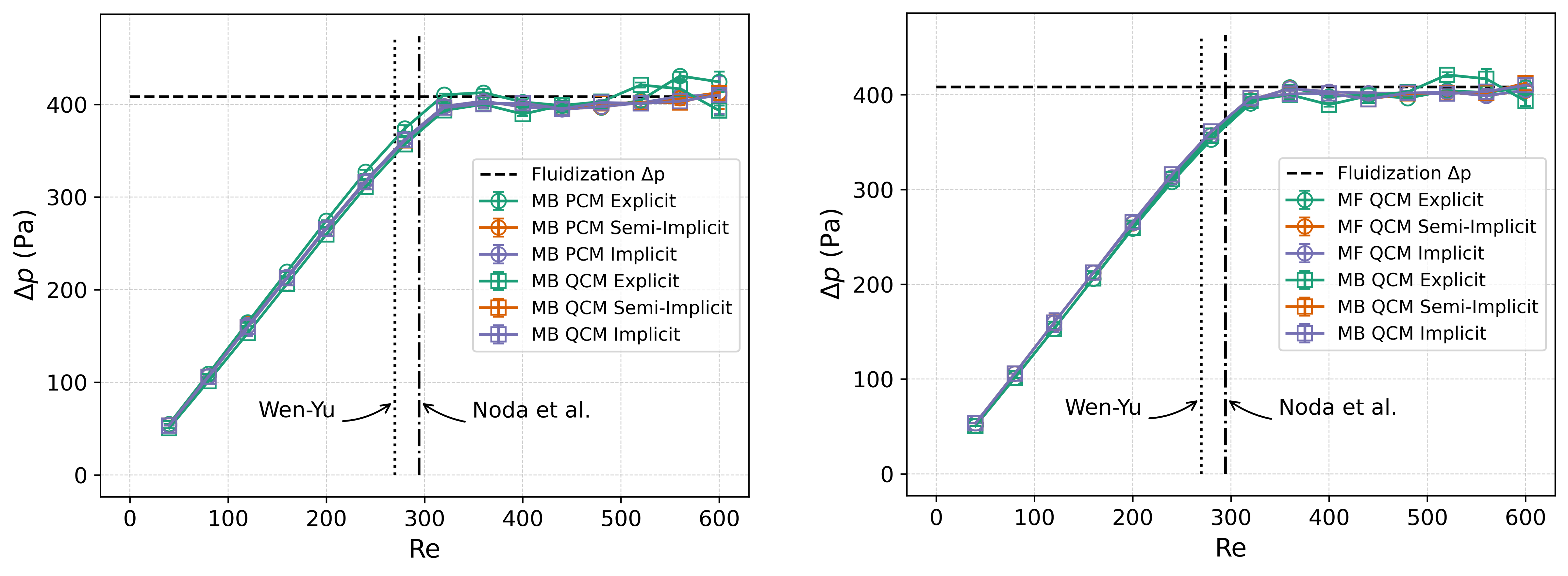
The figure on the left compares the matrix-based (MB) solver results with a cell-based PCM filter and to those with the same solver but a QCM filter. The figure on the right compares the MB solver with the matrix-free (MF) solver results, both obtained with a QCM filter. The different colors correspond to the different drag coupling approaches (explicit in green, semi-implicit in orange, and implicit in purple).

It can be seen that all simulations recover the expected constant pressure-drop plateau after fluidization (shown with the horizontal dashed line), equal to the net weight of the particle bed (weight minus buoyancy) per unit area:

\[\Delta p = \frac{N_\mathrm{p} V_\mathrm{p} (\rho_\mathrm{p}-\rho_\mathrm{f}) g}{A_\mathrm{b}}\]

with \(N_\mathrm{p}\) the number of particles, \(V_\mathrm{p}\) the volume of a particle, and \(A_\mathrm{b}\) the cross-sectional area of the bed.

It can be seen that the increasing portion of the pressure-drop curve is almost identical across the different cases, with the most pronounced deviation observed for the explicit drag coupling using the PCM filter. All curves appear to plateau at a similar \(\mathrm{Re}\), between \(300\) and \(400\), which is close to the minimum fluidization Reynolds number predicted by the Wen–Yu (\(\mathrm{Re}_{\text{mf}}=270\)) and Noda et al. (\(\mathrm{Re}_{\text{mf}}=294\)) correlations. Fluctuations in the pressure-drop values appear after fluidization, generally increasing with increasing \(\mathrm{Re}\). These fluctuations are expected, as the particles become more dynamic, requiring longer sampling times (longer than \(0.05\) s). Differences between the different cases in this region arise from the sensitivity of the particle dynamics to small changes in the different variables, a consequence of the chaotic behavior. Overall, the results demonstrate good agreement between the different solver configurations and with the expected physical behavior of a gas–solid fluidized bed.

References

[1] (1,2)

T. El Geitani, S. Golshan, and B. Blais, “Toward High-Order CFD-DEM: Development and Validation,” Industrial & Engineering Chemistry Research, vol. 62, no. 2, pp. 1141–1159, January 2023. Available: https://doi.org/10.1021/acs.iecr.2c03546.

[2]

C. Wen and Y. Yu, “A generalized method for predicting the minimum fluidization velocity,” AIChE journal, vol. 12, pp. 610–612, May 1966. Available: https://doi.org/10.1002/aic.690120343.

[3]

K. Noda, S. Uchida, T. Makino and H. Kamo, “Minimum fluidization velocity of binary mixture of particles with large size ratio,” Powder Technology, vol. 46, no.2-3, pp. 149–154, April-May 1986. Available: https://doi.org/10.1016/0032-5910(86)80021-3.