Tracer through CAD Junction in Simplex#
In this example, we solve a problem using the simplex capabilities of Lethe. The simplex grids can be generated easily to represent complex geometries, such as a junction of channels made from boolean addition. We will also demonstrate the tracer physics capabilities.
Features#
Solver:
lethe-fluidTransient problem
Displays the use of the tracer physics
Displays the use of a simplex mesh generated with a CAD platform
Files Used in This Example#
All files mentioned below are located in the example’s folder (examples/multiphysics/tracer-through-cad-junction).
Hierarchical Data Format file for SALOME mesh generation:
tracer-through-cad-junction.hdfGMSH geometry file:
tracer-through-cad-junction.geoGMSH mesh file:
tracer-through-cad-junction.mshParameter file:
tracer-through-cad-junction.prmSALOME mesh file:
Mesh-1.mesh
Description of the Case#
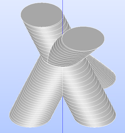
A junction of pipes following an arbitrary path is difficult to mesh properly with hexaedral elements. A simplex mesh, on the other hand, is easy to setup and can be built with many well-established algorithms; all software that can create a mesh can create a simplex mesh. In this example, we consider a junction of pipes that follow orthogonal sinusoids. This case shows how a passive tracer injected in such a geometry can be used to visualize preferential paths.
Generating a Geometry with SALOME#
Complex geometries can be set up and meshed with the SALOME platform.
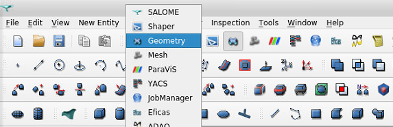
First, the geometry module must be loaded as such, and geometric shapes can be added. For example, here, disks are drawn alongside sinusoidal curves that will be used for pipe generation through extrusion. The Fuse command can then be used to obtain a single geometry.
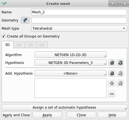
Second, the mesh module can be loaded to generate a .mesh file. A new mesh must be created with an associated geometry, algorithm and hypothesis. NETGEN 1D-2D-3D works well, and automatic hypothesis selection can be used. The element size can be edited to specific requirements, and then the Compute command must be used to generate the grid. Through File -> Export -> GMF File, the .mesh file can be output.
Adding the Boundary IDs from Gmsh#
A criterion for the use of .msh file in Lethe is that the boundaries have an associated ID number. These numbers can be added in Gmsh.
The boundaries from the mesh must be linked to a Physical object. In 3D for example, the inlet, outlet and walls must be specified as Physical surfaces. Selecting the surface for the inlet and outlet can be done easily, and then the .geo file can be text-edited to add a new physical surface with the remaining surfaces.
In this specific case, there are four boundaries: inlets with no tracer (1), inlet with tracer (2), walls (3) and outlets (4), as stated in the .geo file (see excerpt in the text block below).
Merge "Mesh-1.mesh";
Physical Surface(1) = {729, 712};
Physical Surface(2) = {10};
Physical Surface(3) = {1:9,11:711,713:728,730:848,850,852:5000};
Physical Surface(4) = {849, 851};
The Physical Volume must also be specified for compatibility with deal.II, as stated with this line from the .geo file:
Physical Volume(1) = {1};
The last step in Gmsh is to generate the 3D mesh, and then save it to a .msh file.
Parameter File#
Using Lethe requires a solver executable, in this case lethe-fluid, and a .prm file. This second one can be setup in many ways, but for this specific case two aspects must be treated with more care: the enabling of simplex mode, and the setup of the tracer physics.
Enabling the Simplex Mode#
Mesh#
In the subsection mesh, the simplex mode can be enabled with set simplex = true. Also, the mesh in the .msh file must obviously be built with simplex elements.
subsection mesh
  set type               = gmsh
  set file name          = tracer-through-cad-junction.msh
  set initial refinement = 0
  set simplex            = true
end
Warning
If the mesh type is set to dealii instead of gmsh, the deal.II generated mesh will be properly built with simplices.
Warning
[2022-01-19] It is crucial to consider a current limitation : simplex grid refinement isn’t implemented in Lethe.
Setting up the Tracer Physics#
Using the tracer physics requires four elements: activating the physics, setting the tracer diffusivity, setting the tracer elements order and setting the boundary conditions. These elements are provided as such:
Multiphysics#
subsection multiphysics
  set tracer = true
end
Physical Properties#
subsection physical properties
  subsection fluid 0
    set kinematic viscosity = 1
    set tracer diffusivity  = 0.001
  end
end
FEM#
subsection FEM
  set velocity order = 1
  set pressure order = 1
  set tracer order   = 1
end
Tracer Boundary Conditions#
subsection boundary conditions tracer
  set number = 2
  subsection bc 0
    set id   = 1
    set type = dirichlet
    subsection dirichlet
      set Function expression = 0
    end
  end
  subsection bc 1
    set id   = 2
    set type = dirichlet
    subsection dirichlet
      set Function expression = 1
    end
  end
end
The boundary conditions are written in a specific way. We have specified 2 boundaries, a Dirichlet condition with a concentration of 1 for the first inlet, and another Dirichlet condition with a tracer concentration of 0 for the second inlet. All the remaining boundaries are unspecified. An unspecified boundary condition in Lethe for the tracer is considered as the natural condition of finite elements, which is a zero gradient condition.
Note
The boundary conditions tracer subsection is different from the general boundary conditions
which concerns the flow.
Boundary Conditions#
The boundary conditions subsection for the flow is setup as follows. The inlet with a high tracer concentration (id = 2)
is given a higher velocity than the other two (id = 1). The walls of the junction (id = 3) are given a no slip type.
The remaining boundaries (id = 4) are unspecified for the same reason as in the previous subsection: no constraint
must be applied to the outlet flow.
subsection boundary conditions
  set number = 3
  subsection bc 0
    set id   = 1
    set type = function
    subsection u
      set Function expression = 0
    end
    subsection v
      set Function expression = 0
    end
    subsection w
      set Function expression = 1
    end
  end
  # boundary id2 will have the tracer
  subsection bc 1
    set id   = 2
    set type = function
    subsection u
      set Function expression = 0
    end
    subsection v
      set Function expression = 0
    end
    subsection w
      set Function expression = 4
    end
  end
  subsection bc 2
    set id   = 3
    set type = noslip
  end
end
Running the Simulation#
The case must be run with the solver and the parameter file. The simulation is launched in the same folder as the .prm file, using the lethe-fluid solver. It takes a long time since problem is transient and the time steps are short. Assuming that the lethe-fluid executable is within your path, the simulation can be launched by typing:
Results#
The results in .pvd format can then be viewed using visualisation software such as Paraview.
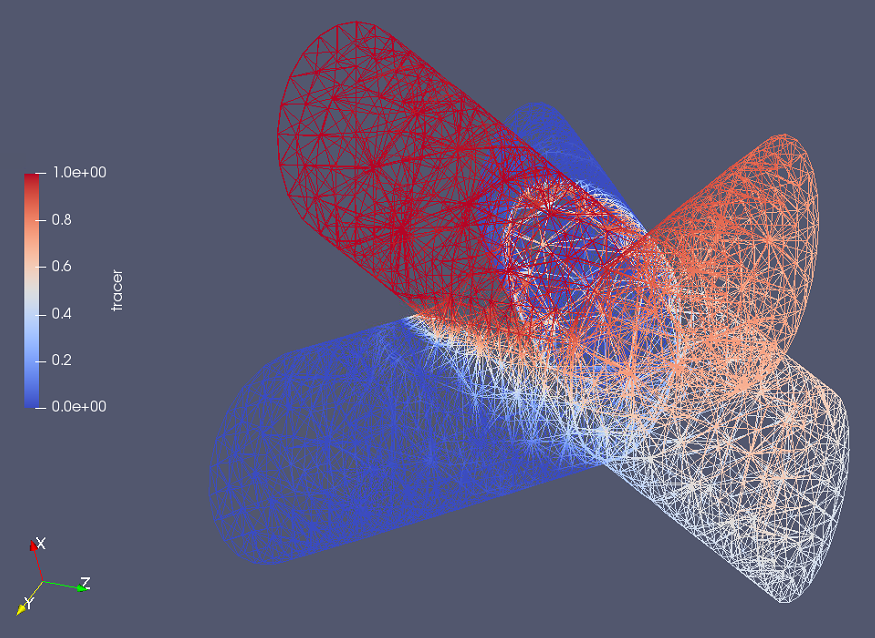
The higher presence of tracer in the outlet on the same side as the tracer inlet may indicate poor mixing. As the tracer diffusivity is low, the mixing between the streams comes mainly from advection. However, since the kinematic viscosity is high, the flow is laminar (i.e. dominated by viscous forces) and the streamlines do not cross.