Laser Melt Pool

This example simulates a two-dimensional melt pool with a laser [1].

Features

• Solver: lethe-fluid

• Laser heat source

• Phase change (solid-liquid)

• Buoyant force (natural convection)

• Convection-radiation heat transfer boundary condition

• Unsteady problem handled by an adaptive BDF2 time-stepping scheme

• Mesh adaptation using temperature

Files Used in This Example

• Parameter file: examples/multiphysics/laser-melt-pool/laser-melt-pool.prm

Description of the Case

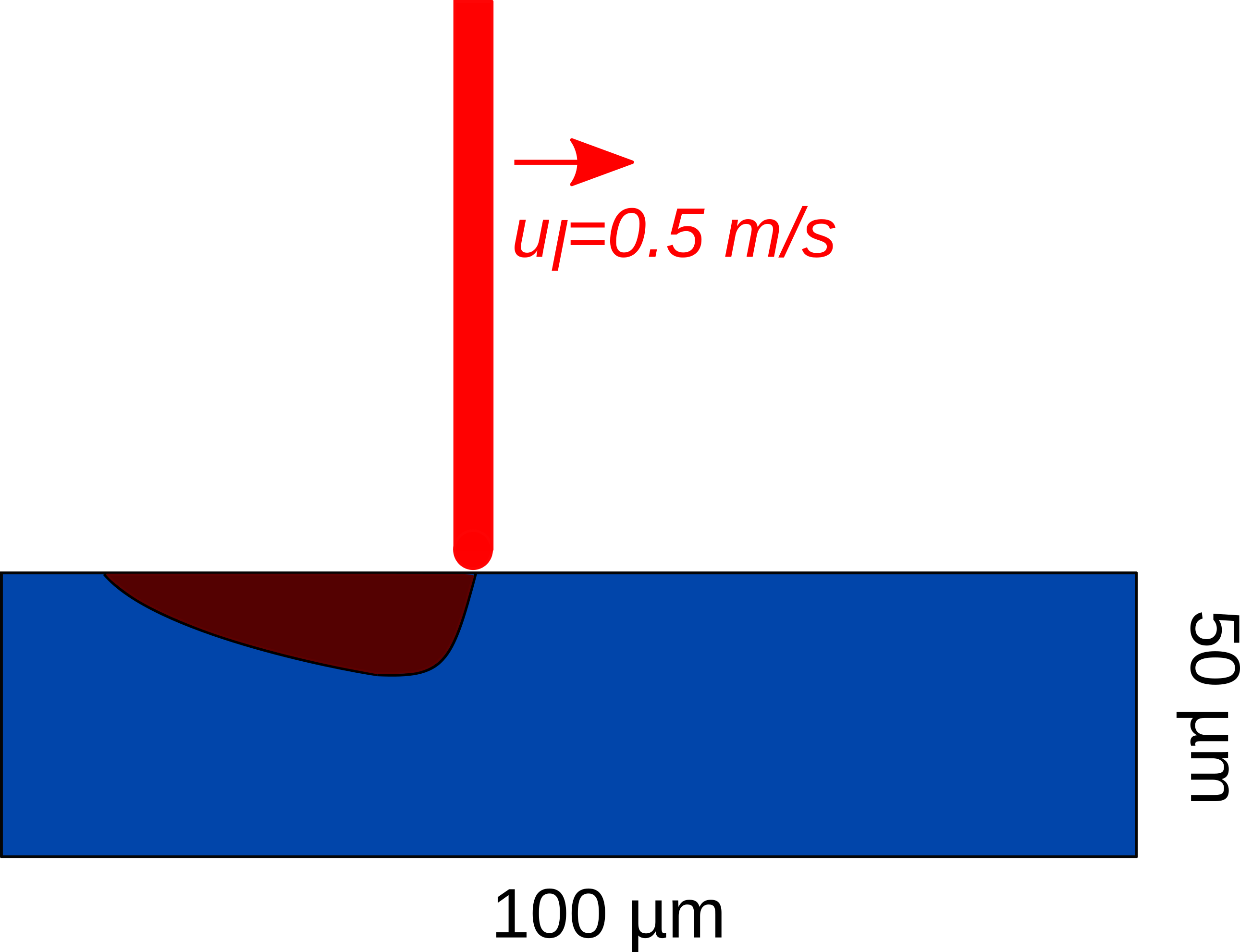
A Ti-6Al-4 V powder bed (assumed as a solid block in this example) melts using a laser beam that is emitted perpendicular to the top surface of the block. The laser beam speed is 0.5 m/s. Due to the laser heat source, the solid block melts in the direction of the laser. The corresponding parameter file is laser-melt-pool.prm.

The following schematic describes the geometry and dimensions of the simulation in the \((x,y)\) plane:

Parameter File

Time integration is handled by a 2nd order backward differentiation scheme (bdf2) (for a better temporal accuracy), for a \(0.005\) seconds simulation time with a constant time step of \(5.0 \times 10^{-6}\) seconds.

Simulation Control

subsection simulation control
  set method           = bdf2
  set time end         = 0.005
  set time step        = 0.000005
  set output name      = laser-melt-pool
  set output frequency = 1
  set output path      = ./output/
end

Boundary Conditions

All the four boundary conditions are noslip, and the heat transfer boundary conditions are convection-radiation-flux with a convective heat transfer coefficient of 80 \(\text{W}\text{m}^{-2}\text{K}^{-1}\), ambient temperature is 20 \(^{\circ}\text{C}\), and emissivity is 0.6.

subsection boundary conditions
  set number = 4
  subsection bc 0
    set id   = 0
    set type = noslip
  end
  subsection bc 1
    set id   = 1
    set type = noslip
  end
  subsection bc 2
    set id   = 2
    set type = noslip
  end
  subsection bc 3
    set id   = 3
    set type = noslip
  end
end
subsection boundary conditions heat transfer
  set number = 4
  subsection bc 0
    set id         = 0
    set type       = convection-radiation-flux
    subsection h
      set Function expression = 80
    end
    subsection Tinf
      set Function expression = 20
    end
    subsection emissivity
      set Function expression = 0.6
    end
  end
  subsection bc 1
    set id         = 1
    set type       = convection-radiation-flux
    subsection h
      set Function expression = 80
    end
    subsection Tinf
      set Function expression = 20
    end
    subsection emissivity
      set Function expression = 0.6
    end
  end
  subsection bc 2
    set id         = 2
    set type       = convection-radiation-flux
    subsection h
      set Function expression = 80
    end
    subsection Tinf
      set Function expression = 20
    end
    subsection emissivity
      set Function expression = 0.6
    end
  end
  subsection bc 3
    set id         = 3
    set type       = convection-radiation-flux
    subsection h
      set Function expression = 80
    end
    subsection Tinf
      set Function expression = 20
    end
    subsection emissivity
      set Function expression = 0.6
    end
  end
end

Multiphysics

The multiphysics subsection enables to turn on (true) and off (false) the physics of interest. Here heat transfer, buoyancy force, and fluid dynamics are enabled.

subsection multiphysics
  set heat transfer  = true
  set buoyancy force = true
  set fluid dynamics = true
end

Laser Parameters

In the laser parameters section, the parameters of the laser model are defined. The exponential decaying model [2] is used to simulate the laser heat source. In the exponential decaying model, the laser heat flux is calculated using the following equation:

\[q(x,y,z) = \frac{\eta \alpha P}{\pi r^2 \mu} \exp{\left(-\eta \frac{r^2}{R^2}\right)} \exp{\left(- \frac{|z|}{\mu}\right)}\]

where \(\eta\), \(\alpha\), \(P\), \(R\), \(\mu\), \(r\) and \(z\) denote concentration factor, absorptivity, laser power, beam radius, penetration depth, radial distance from the laser focal point, and axial distance from the laser focal point, respectively. These parameters are explained in more detail in laser parameters.

Note

The scanning path of the laser is defined using a Function expression in the path subsection.

subsection laser parameters
  set enable               = true
  set type                 = exponential_decay
  set concentration factor = 2
  set power                = 100
  set absorptivity         = 0.6
  set penetration depth    = 0.000070
  set beam radius          = 0.000050
  set start time           = 0
  set end time             = 0.001
  set beam orientation     = y-
  subsection path
    set Function expression = 0.5 * t; 0.000500
  end
end

Physical Properties

The laser heat source locally melts the material, which is initially in the solid phase according to the definition of the solidus temperature. Hence, the physical properties should be defined using phase_change models. Interested readers may find more information on phase change model in the Stefan problem example . In the physical properties subsection, the physical properties of the different phases of the fluid are defined:

subsection physical properties
  set number of fluids = 1
  subsection fluid 0
    set thermal conductivity model = phase_change
    set thermal expansion model    = phase_change
    set rheological model          = phase_change
    set specific heat model        = phase_change

    set density = 4420

    subsection phase change
      # Enthalpy of the phase change
      set latent enthalpy = 286000

      # Temperature of the liquidus
      set liquidus temperature = 1650

      # Temperature of the solidus
      set solidus temperature = 1604

      # Specific heat of the liquid phase
      set specific heat liquid = 831

      # Specific heat of the solid phase
      set specific heat solid = 670

      # Kinematic viscosity of the liquid phase
      set viscosity liquid = 0.00000069

      # Kinematic viscosity of the solid phase
      set viscosity solid = 0.008

      set thermal conductivity solid  = 33.4
      set thermal conductivity liquid = 10.6

      set thermal expansion liquid = 0.0002
      set thermal expansion solid  = 0.0
    end
  end
end

Note

Using a phase_change model for the thermal conductivity, the thermal conductivity of the material varies linearly between thermal conductivity solid and thermal conductivity liquid when the temperature is in the range of the solidus and liquidus temperatures.

Mesh

We start the simulation with a rectangular mesh that spans the domain defined by the corner points situated at \([-0.0001, 0]\) and \([0.0009, 0.0005]\). The first \([4,2]\) couple of the set grid arguments parameter defines the number of initial grid subdivisions along the length and height of the rectangle. This allows for the initial mesh to be composed of perfect squares. We proceed then to redefine the mesh globally seven times by setting set initial refinement=7.

subsection mesh
  set type               = dealii
  set grid type          = subdivided_hyper_rectangle
  set grid arguments     = 4, 2 : -0.0001, 0 : 0.0009, 0.000500 : true
  set initial refinement = 7
end

Running the Simulation

Call the lethe-fluid by invoking:

mpirun -np 12 lethe-fluid laser-melt-pool.prm

to run the simulation using twelve CPU cores. Feel free to use more.

Warning

Make sure to compile lethe in Release mode and run in parallel using mpirun. This simulation takes \(\approx\) 3 hours on 12 processes.

Results

The following animation shows the temperature distribution in the simulations domain, as well the melted zone (using white contour lines at the liquidus and solidus temperatures).

References

[1]

E. Li, Z. Zhou, L. Wang, Q. Zheng, R. Zou, and A. Yu, “Melt pool dynamics and pores formation in multi-track studies in laser powder bed fusion process,” Powder Technol., vol. 405, p. 117533, Jun. 2022, doi: 10.1016/j.powtec.2022.117533.

[2]

S. Liu, H. Zhu, G. Peng, J. Yin, and X. Zeng, “Microstructure prediction of selective laser melting AlSi10Mg using finite element analysis,” Mater. Des., vol. 142, pp. 319–328, Mar. 2018, doi: 10.1016/j.matdes.2018.01.022.